7Hello Everyone!!

About SARA

SARA stands for Savitribai Ramabai Institute of Data Science.
It is a Charitable Education Trust, est. in 2023 by Dr. Ajay Kumar Koli & Dr. Kiran Lata Koli.
Our mission to enhance the representation of under-privileged communities in the field of data science.
Work

We think we work like this but …
Work
This is our work look actually.

🤯 Work Flowchart
MS Word
Excel
PPTs
Other Tools:
PDF
SPSS
SAS
STATA
Reference management
Work Influencer

👀 Focus on Content.
💅 Set Yourself Apart.
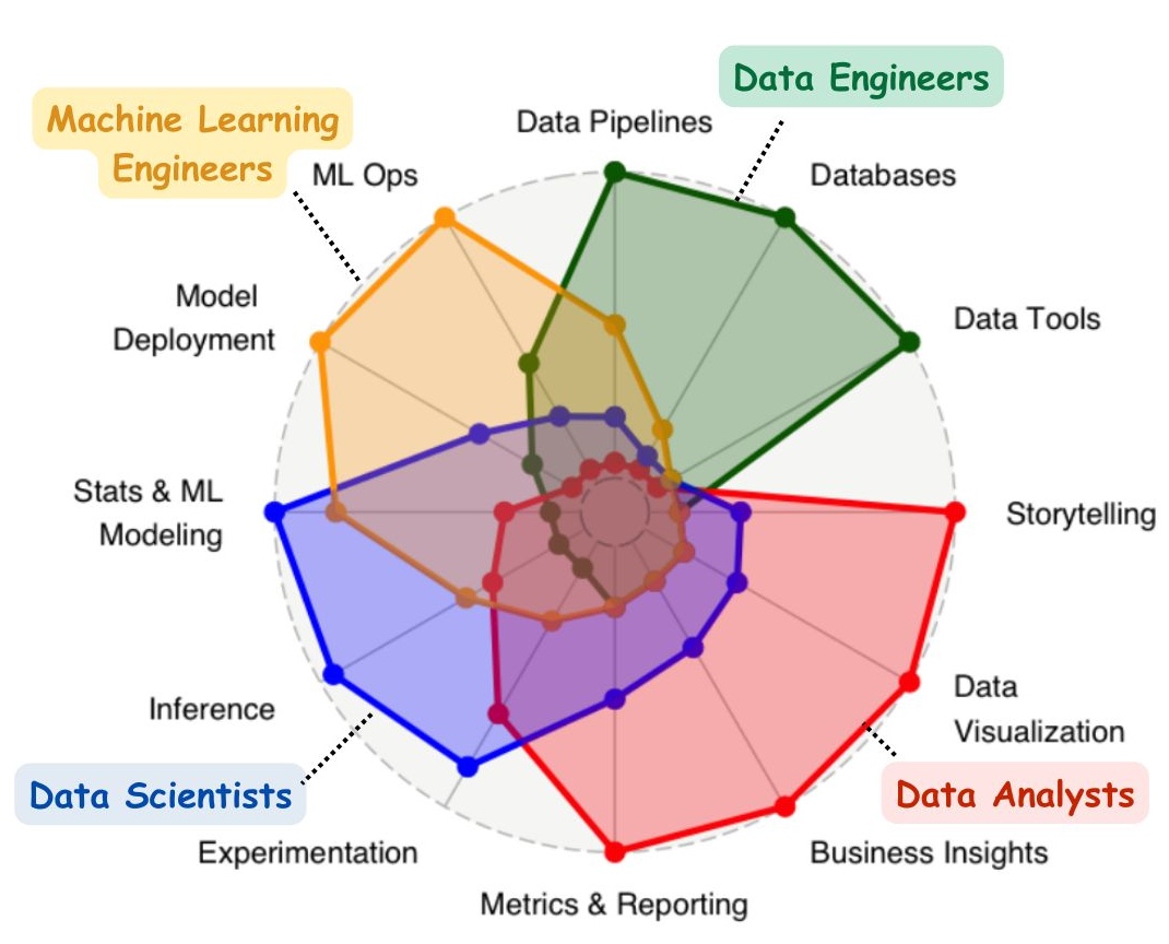
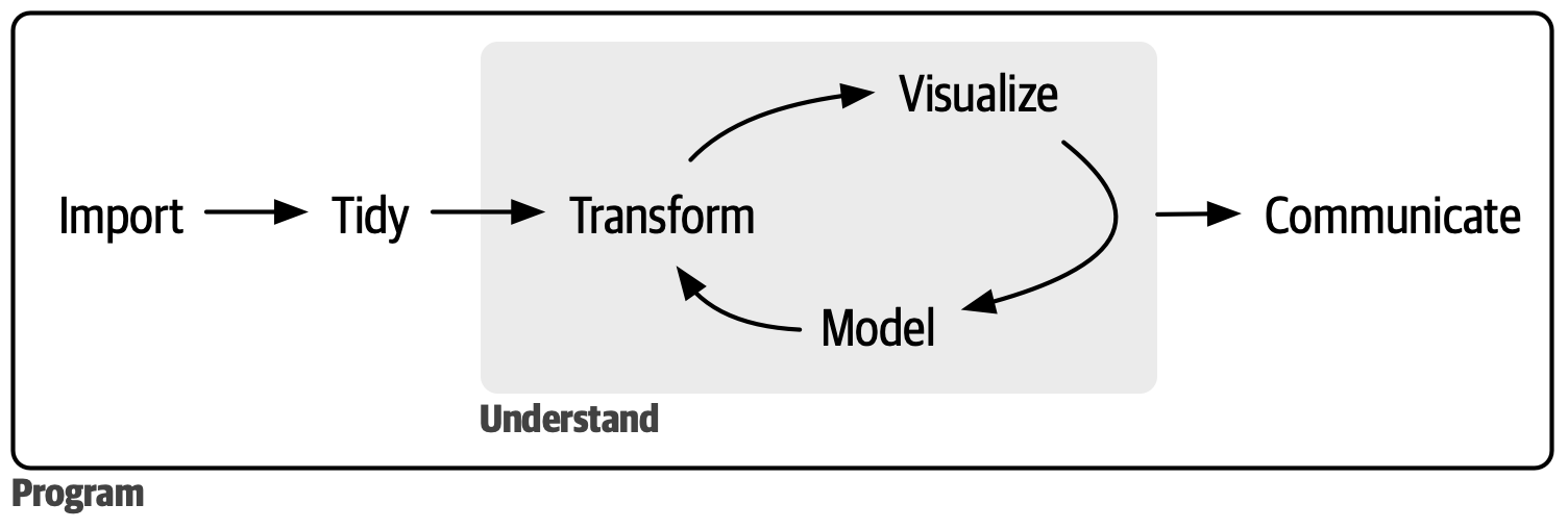
Types of Data Roles
Data Science Process
R Programming Language
![]()
“R is a free software environment for statistical computing and graphics.”
History of R
Initially developed as S language by Bells Labs.
First appeared in August 1993 as R language by:
Ross Ihaka
(New Zealand Statistician)

Robert Gentleman
(Canadian Statistician)

R is FREE
Download R from CRAN

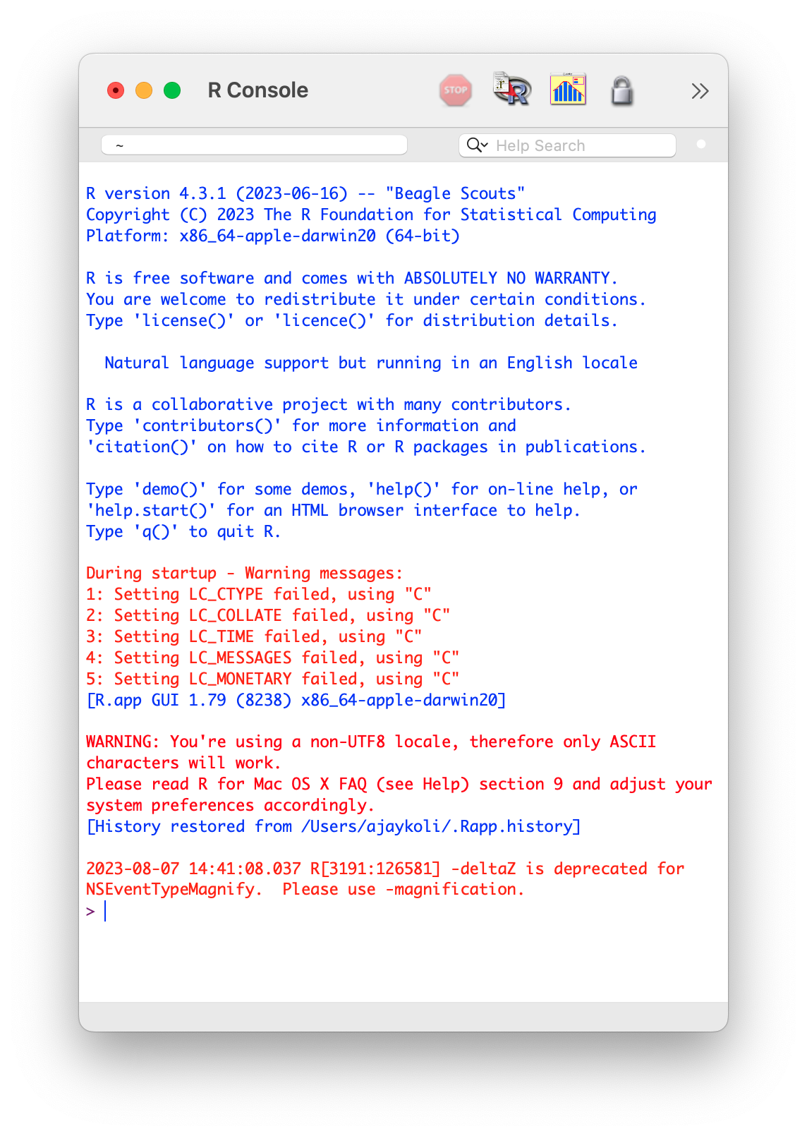
R Console
R version 4.3.1 (2023-06-16)
R name “Beagle Scouts”
R licence “ABSOLUTELY NO WARRANTY”
R prompt
>|
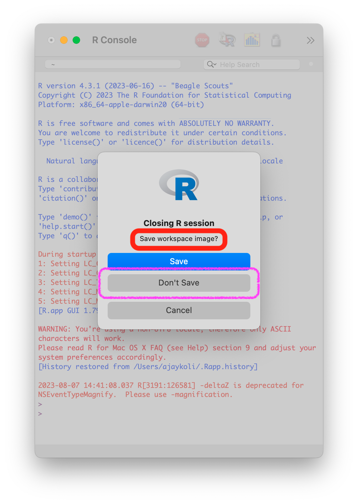
Workspace Image
Don’t save workspace image.
It helps in “freshly minted R sessions”.
“put more trust in your script than in your memory”.
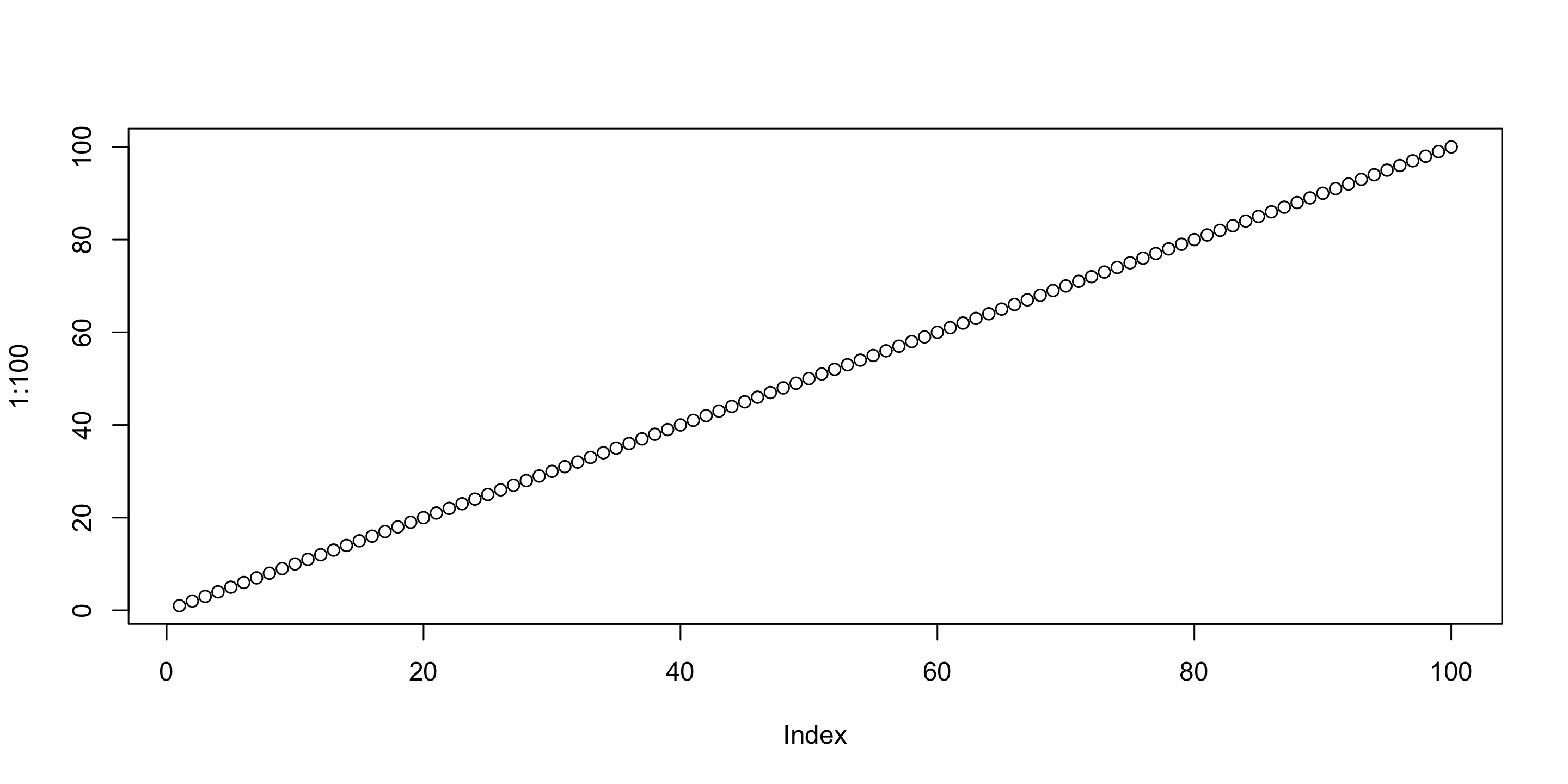
Plot Using R
🔥 WE NEED A SUPERHERO 🔥

![]()
S T U D I O
posit, earlier RStudio
RStudio is an integrated development environment (IDE) for R and Python.
As per posit, RStudio is “the most trusted IDE for open source data science”.
Download RStudio.
![]()
![]()
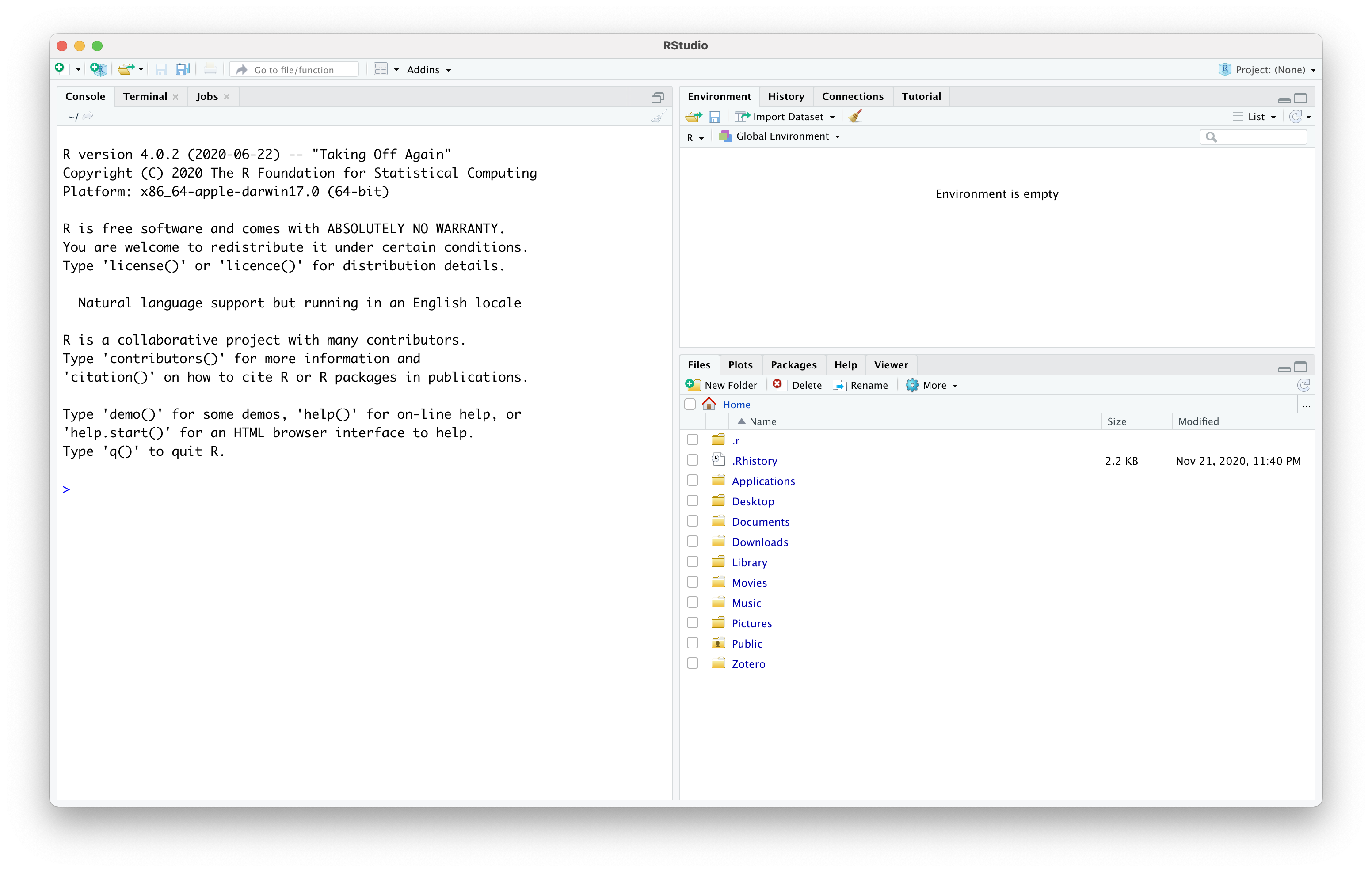
RStudio IDE

RStudio IDE
“It includes a console, syntax-highlighting editor that supports direct code execution, and tools for plotting, history, debugging, and workspace management.”
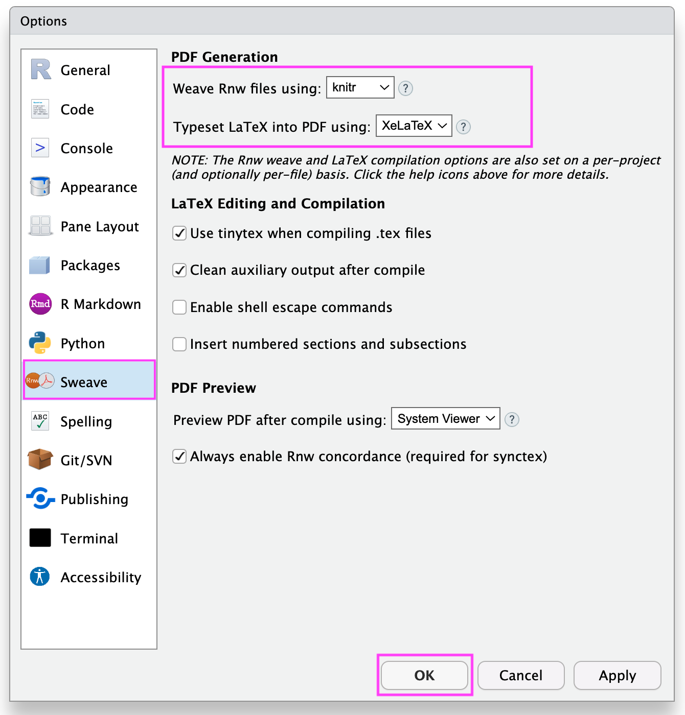
RStudio \(\rightarrow\) Tools \(\rightarrow\) Global Options
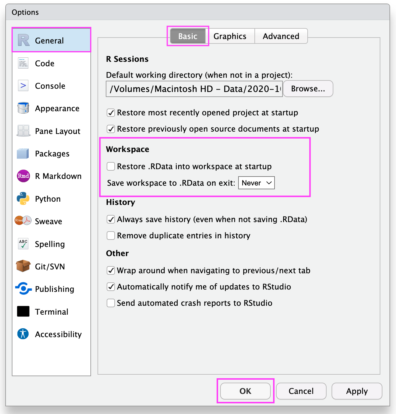
RStudio \(\rightarrow\) Tools \(\rightarrow\) Global Options
PROJECT
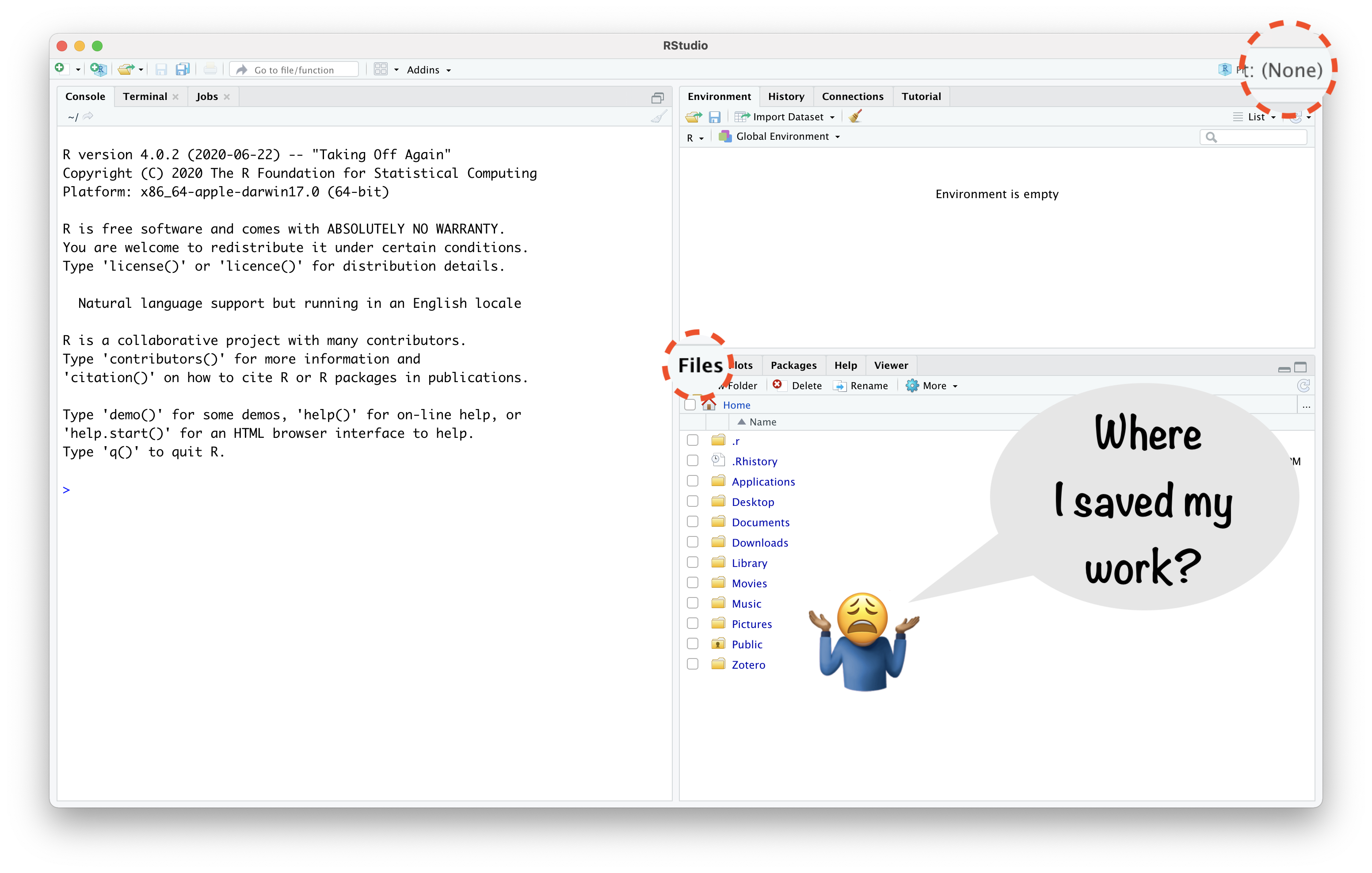
Open RStudio
RStudio Without Project
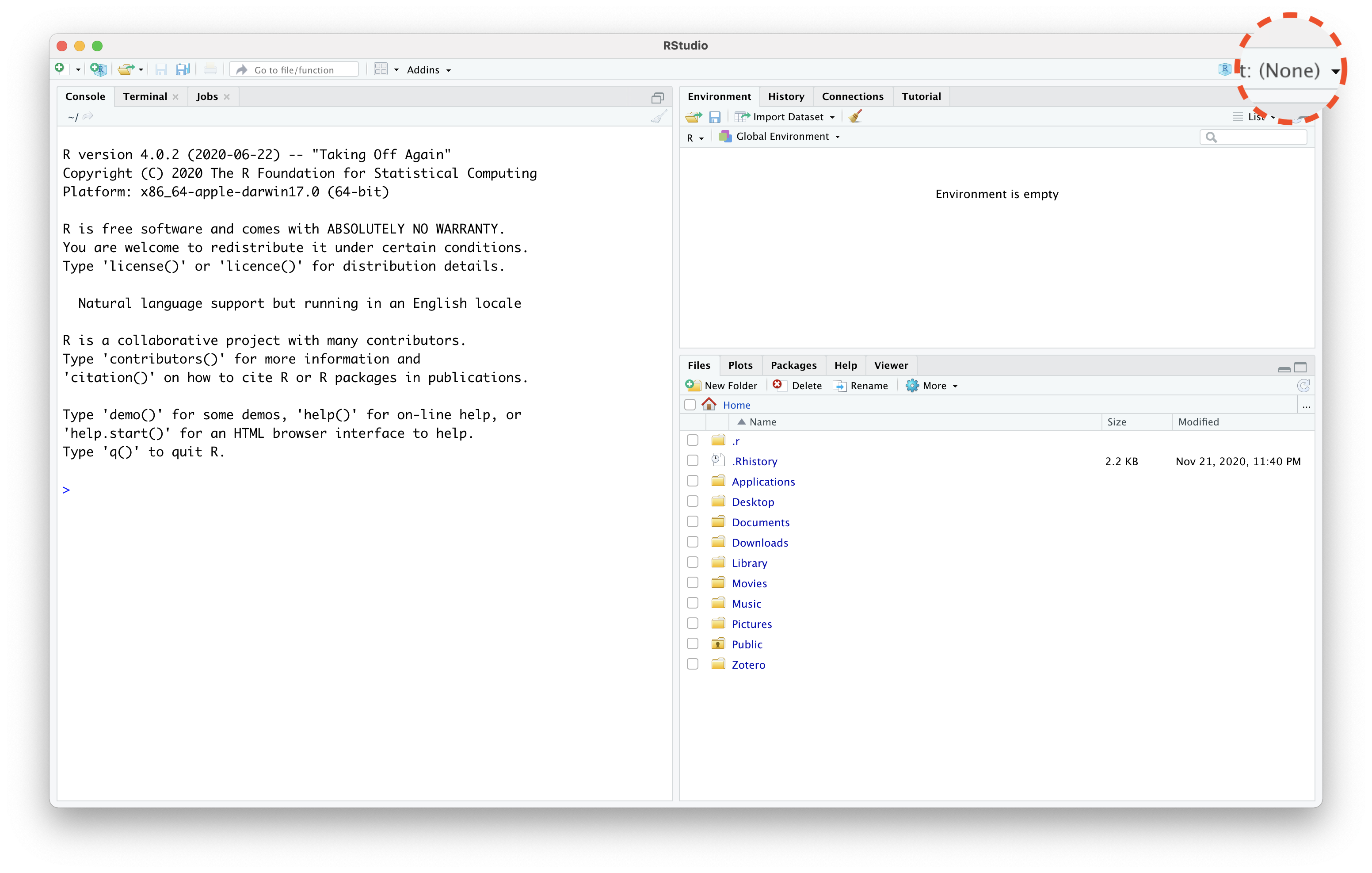
RStudio Without Project
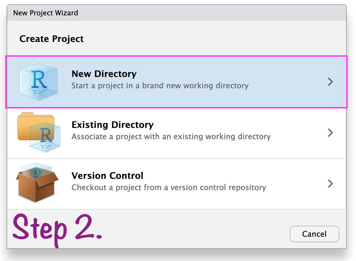
Create RStudio Project

Create RStudio Project
In Case Anything Goes Wrong\(...\)

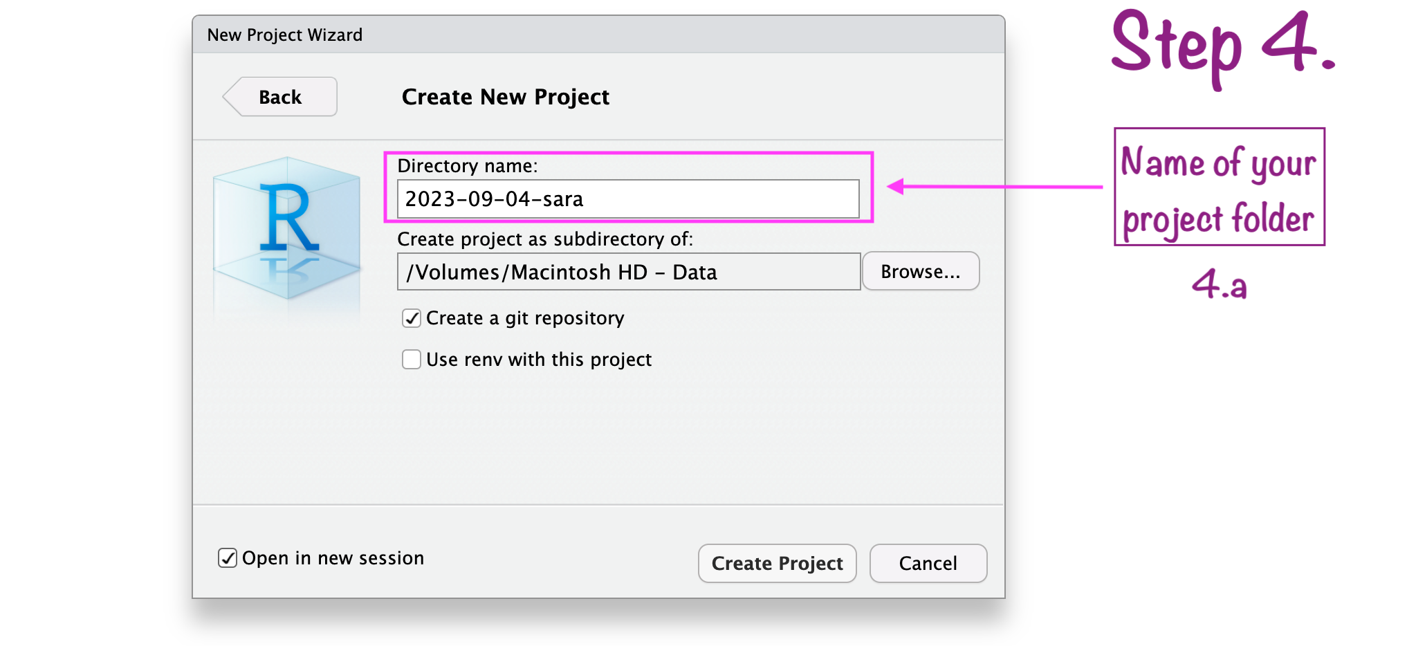
Create RStudio Project
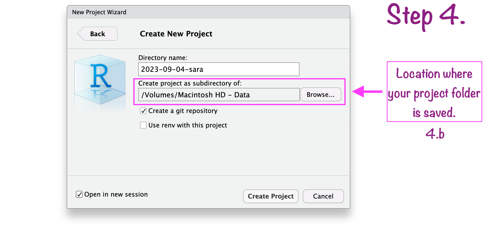
Create RStudio Project
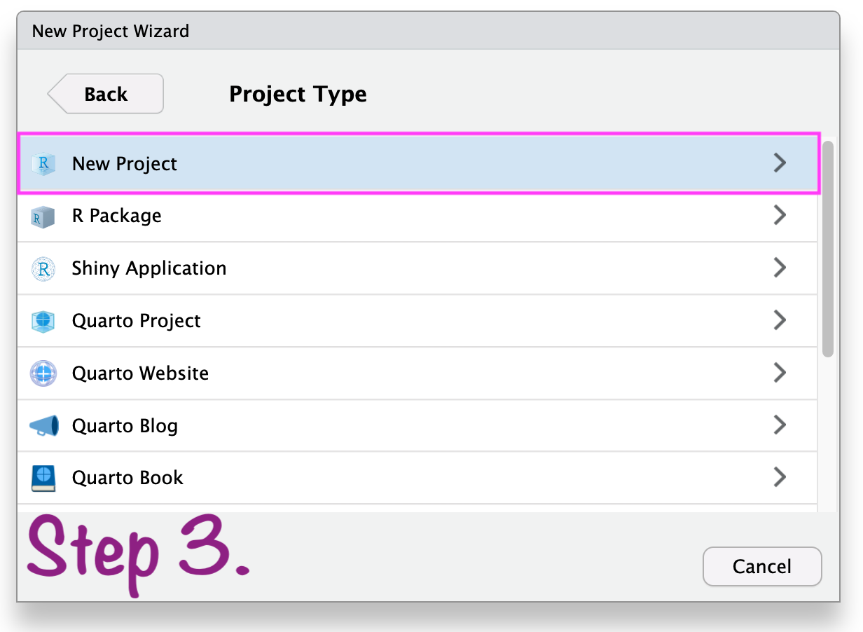
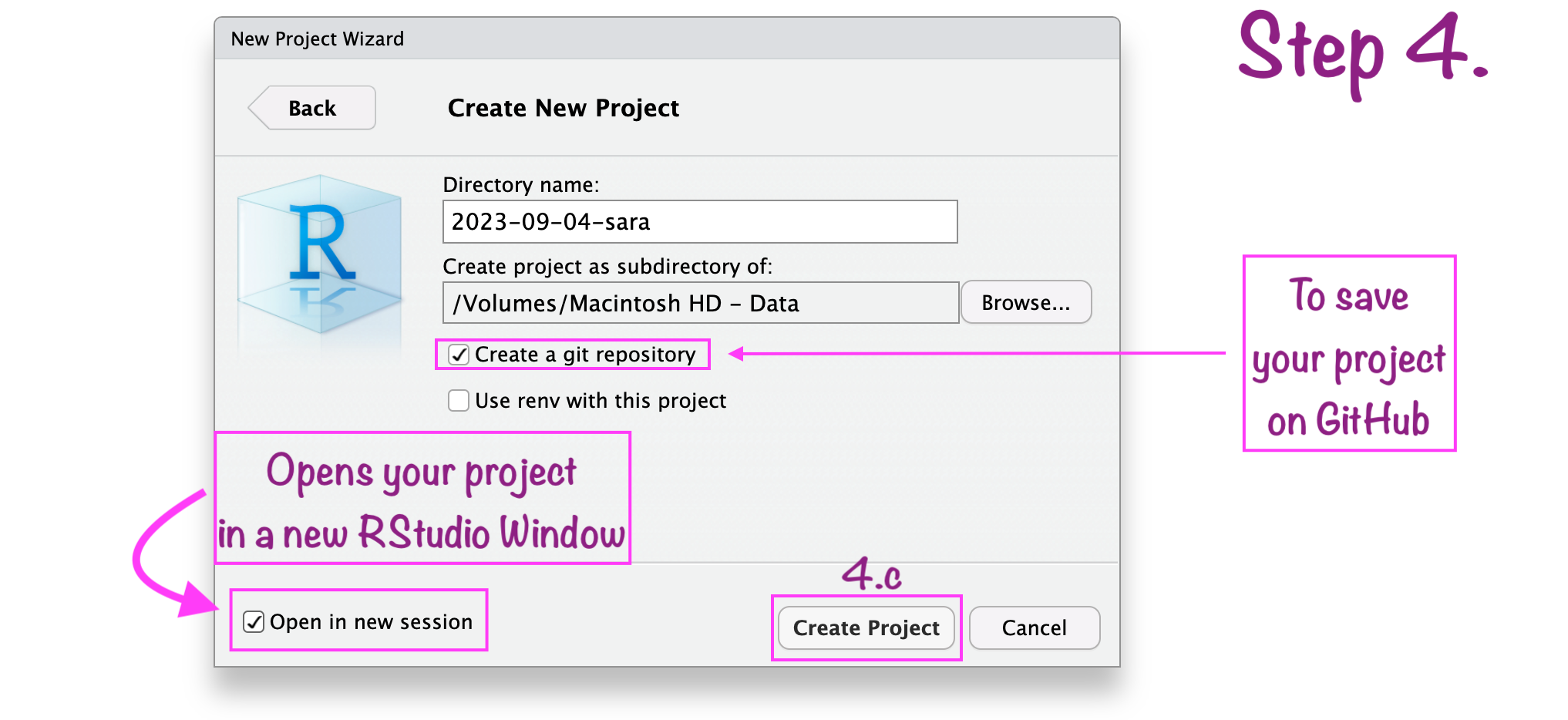
Create RStudio Project
Create RStudio Project
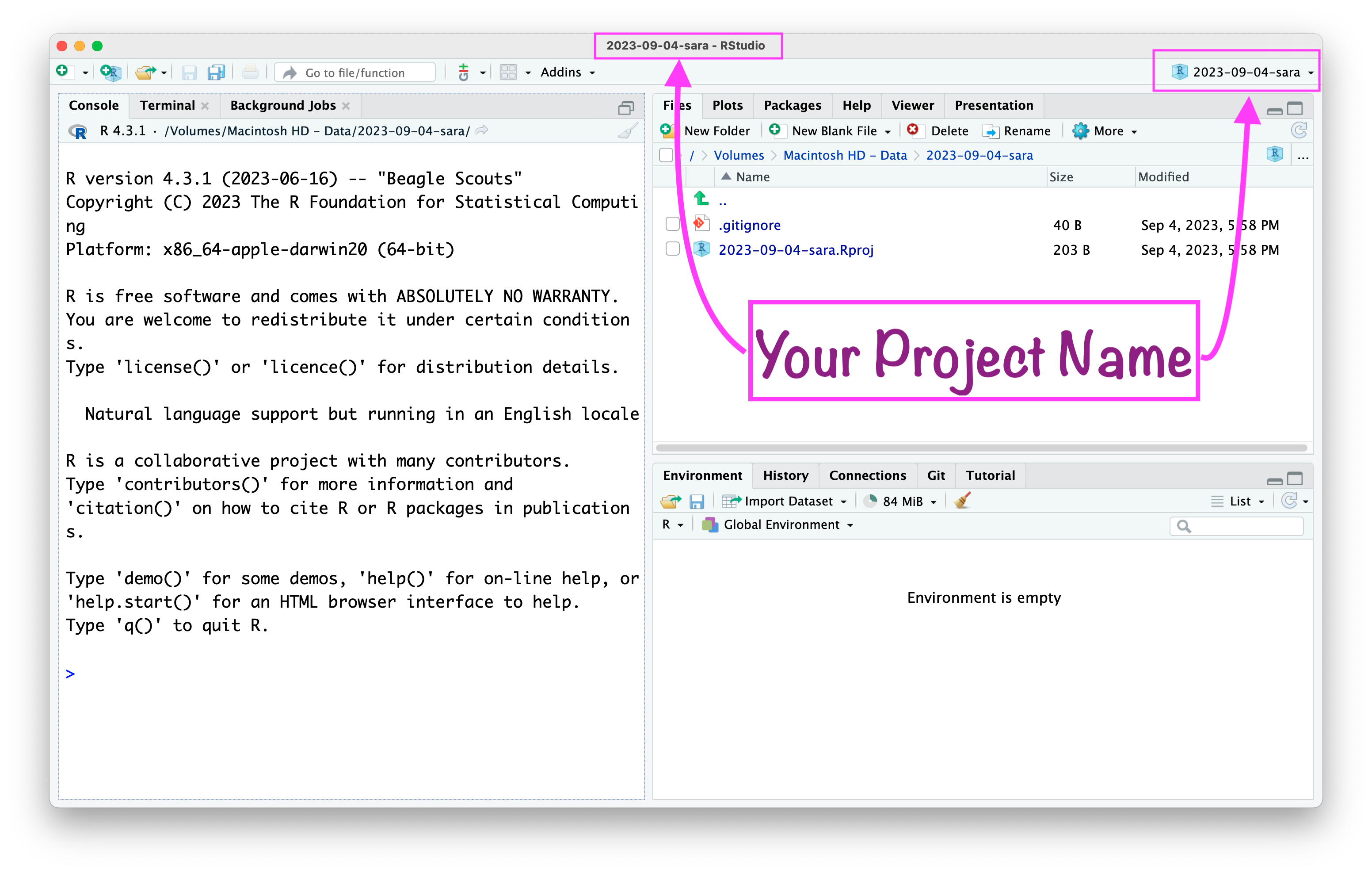
Create RStudio Project
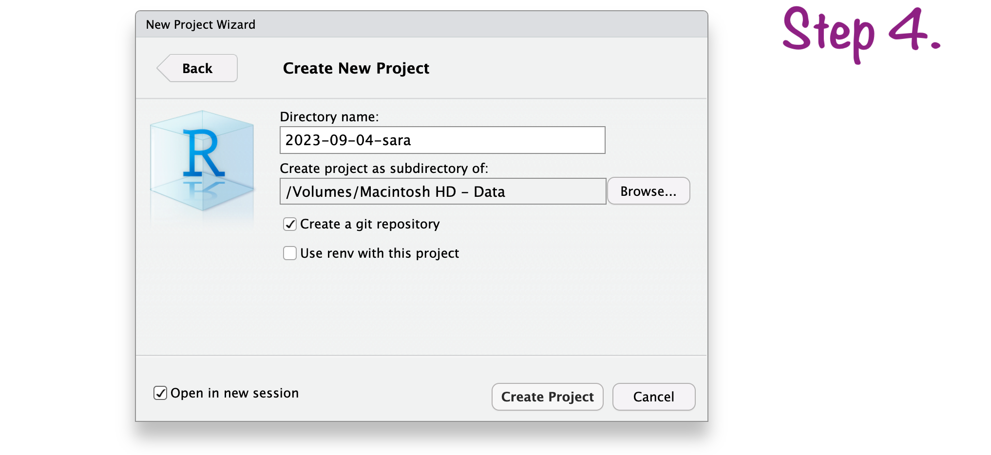
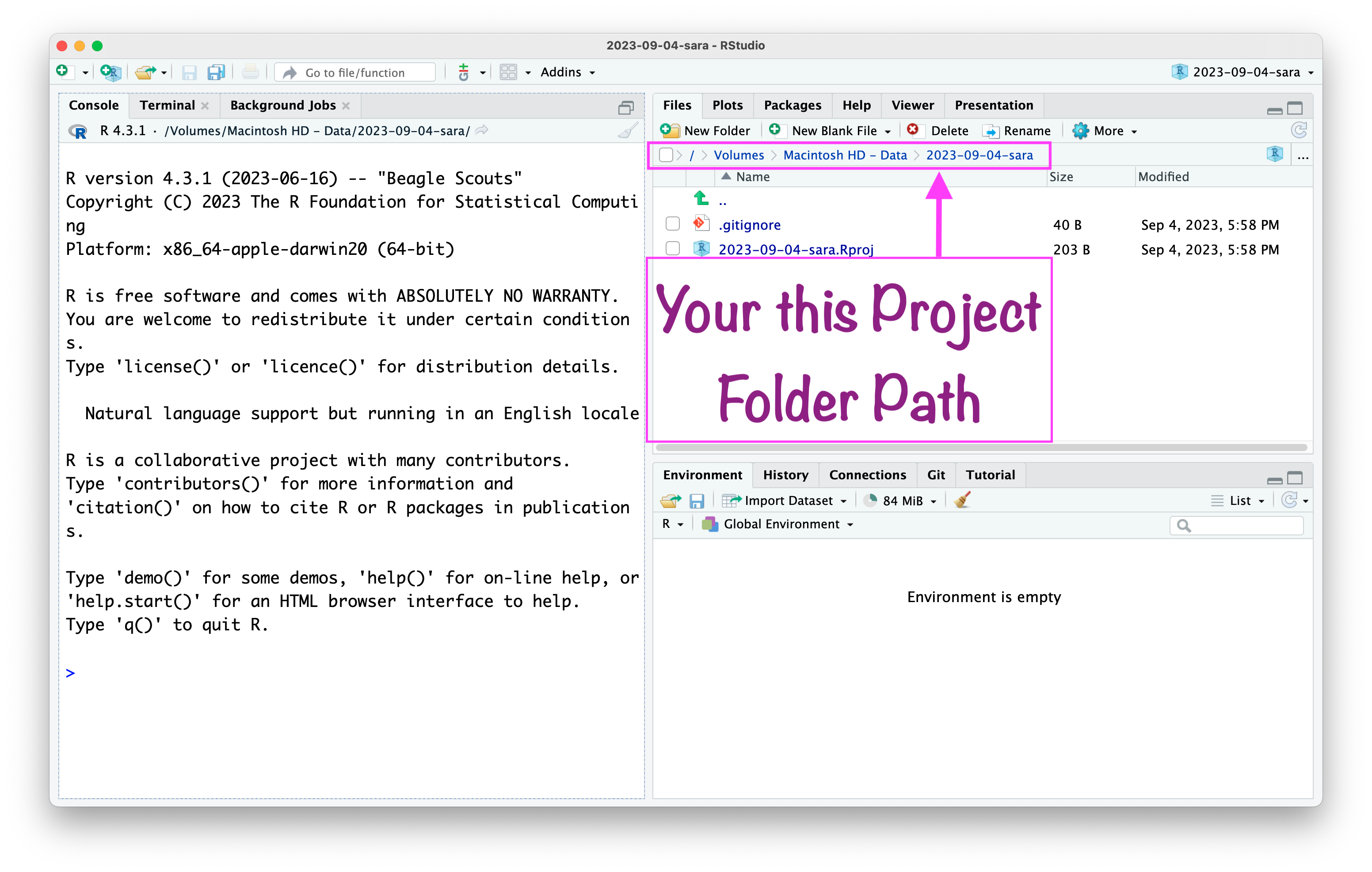
RStudio Project “name”
RStudio Project “path”
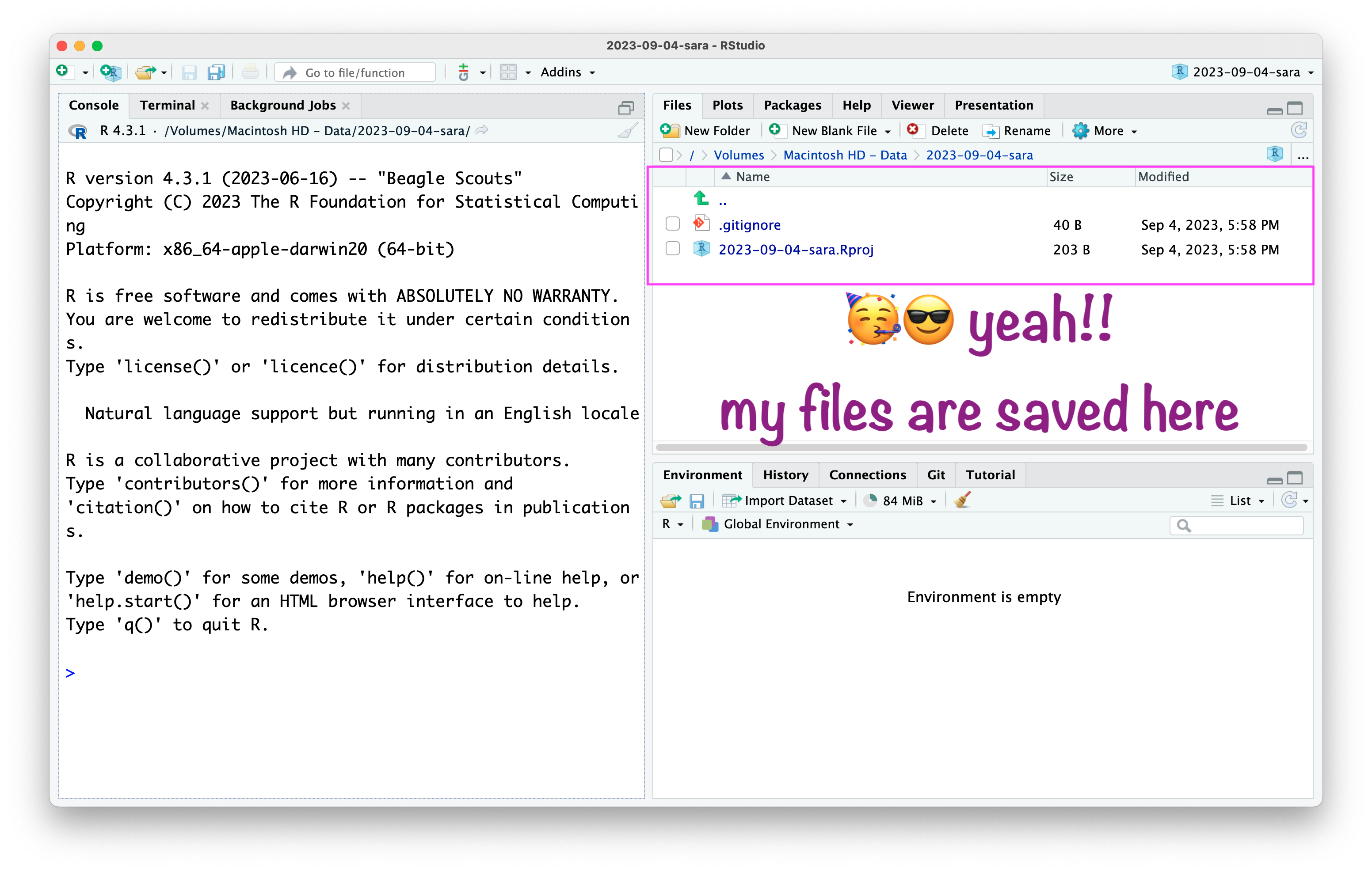
RStudio Project

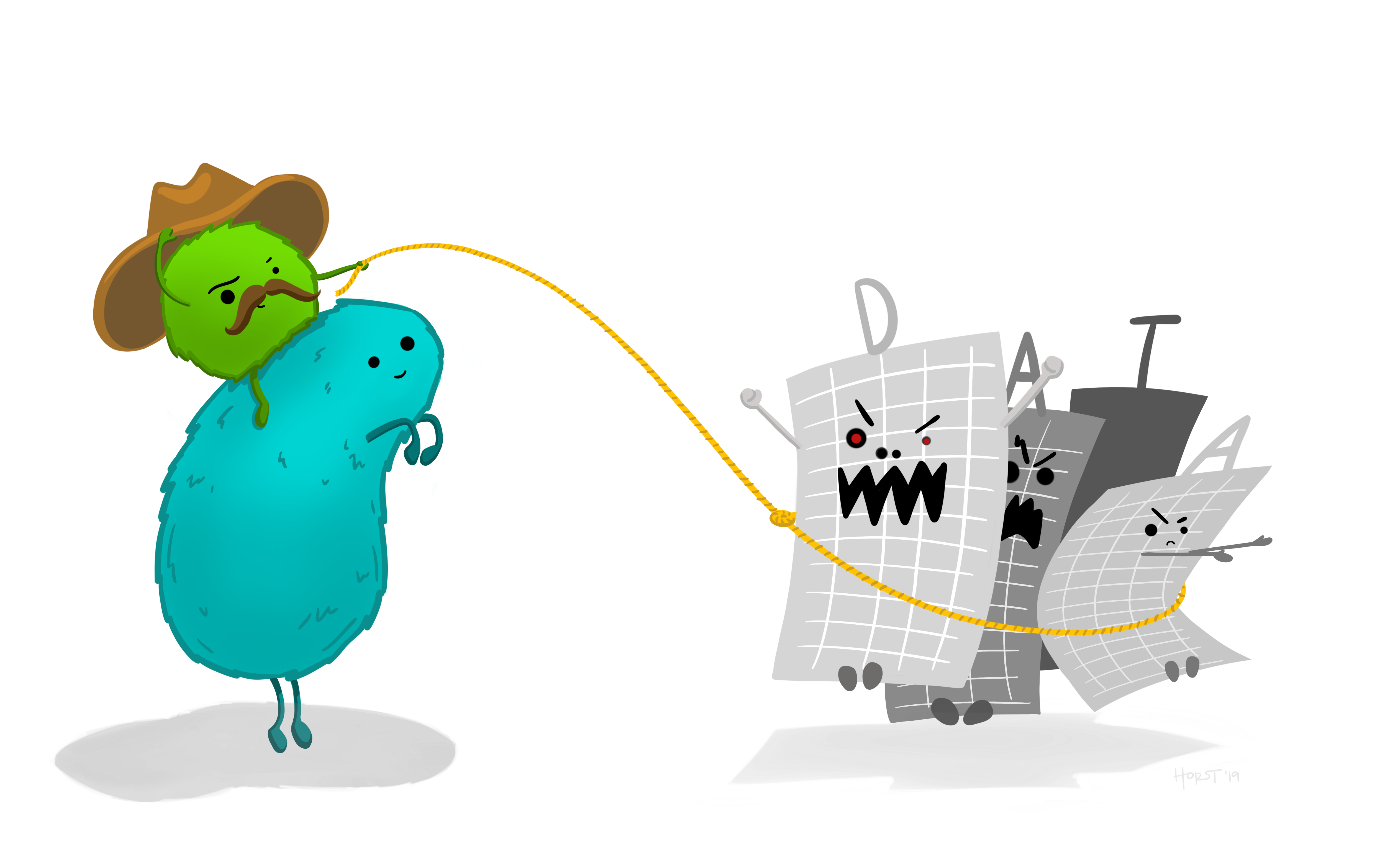
Artwork by Alision Horst
Write R Codes in
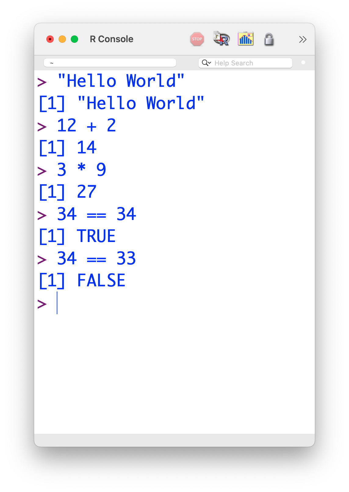
R Console
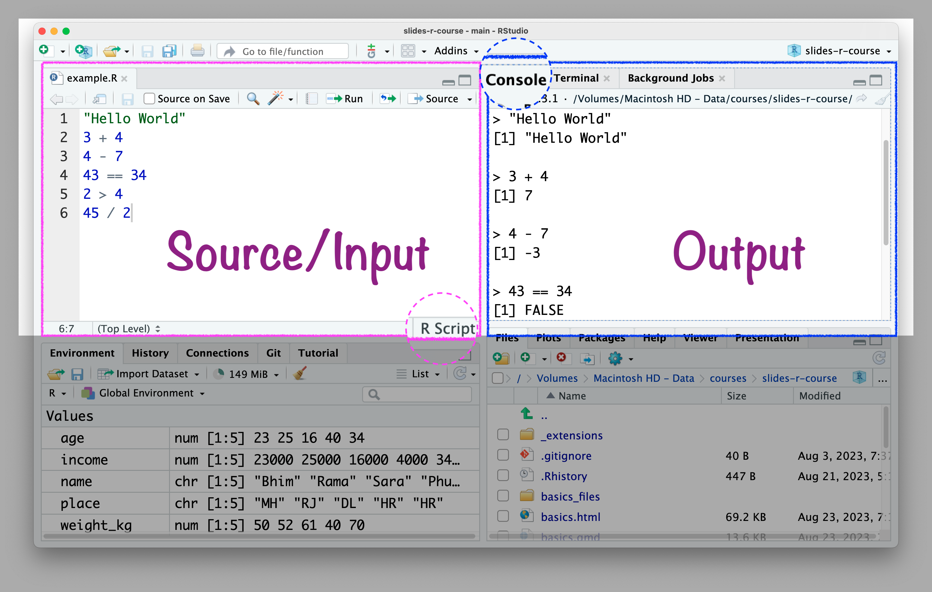
Write R Codes in
R script using RStudio.
Write R Codes in
Quarto document using RStudio
 :::
:::

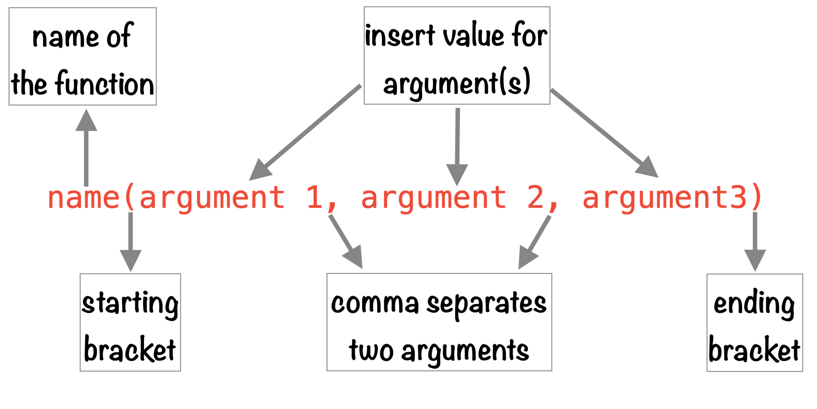
FUNCTION
Artwork by Alision Horst
Structure of R Function
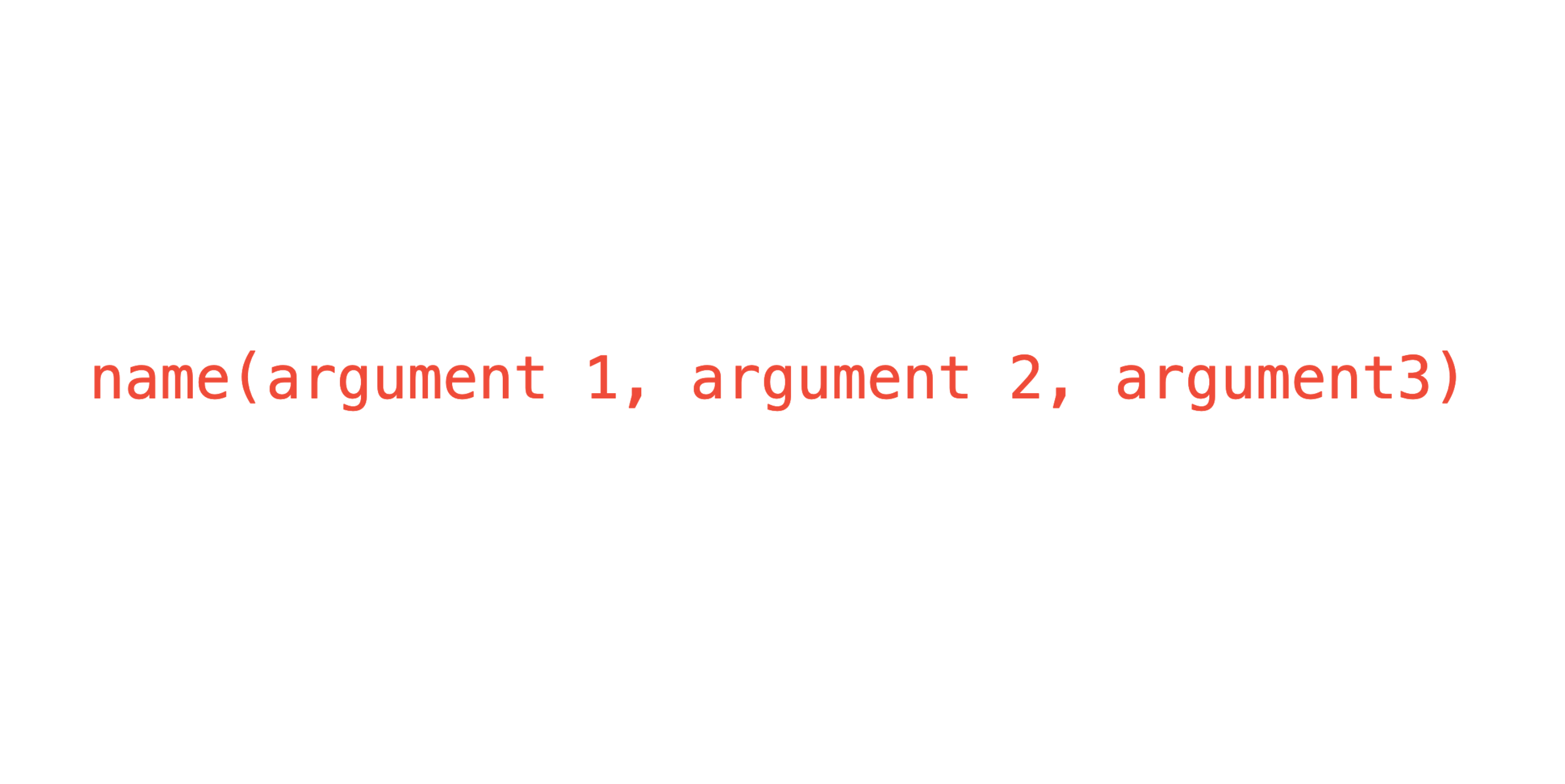
Structure of R Function
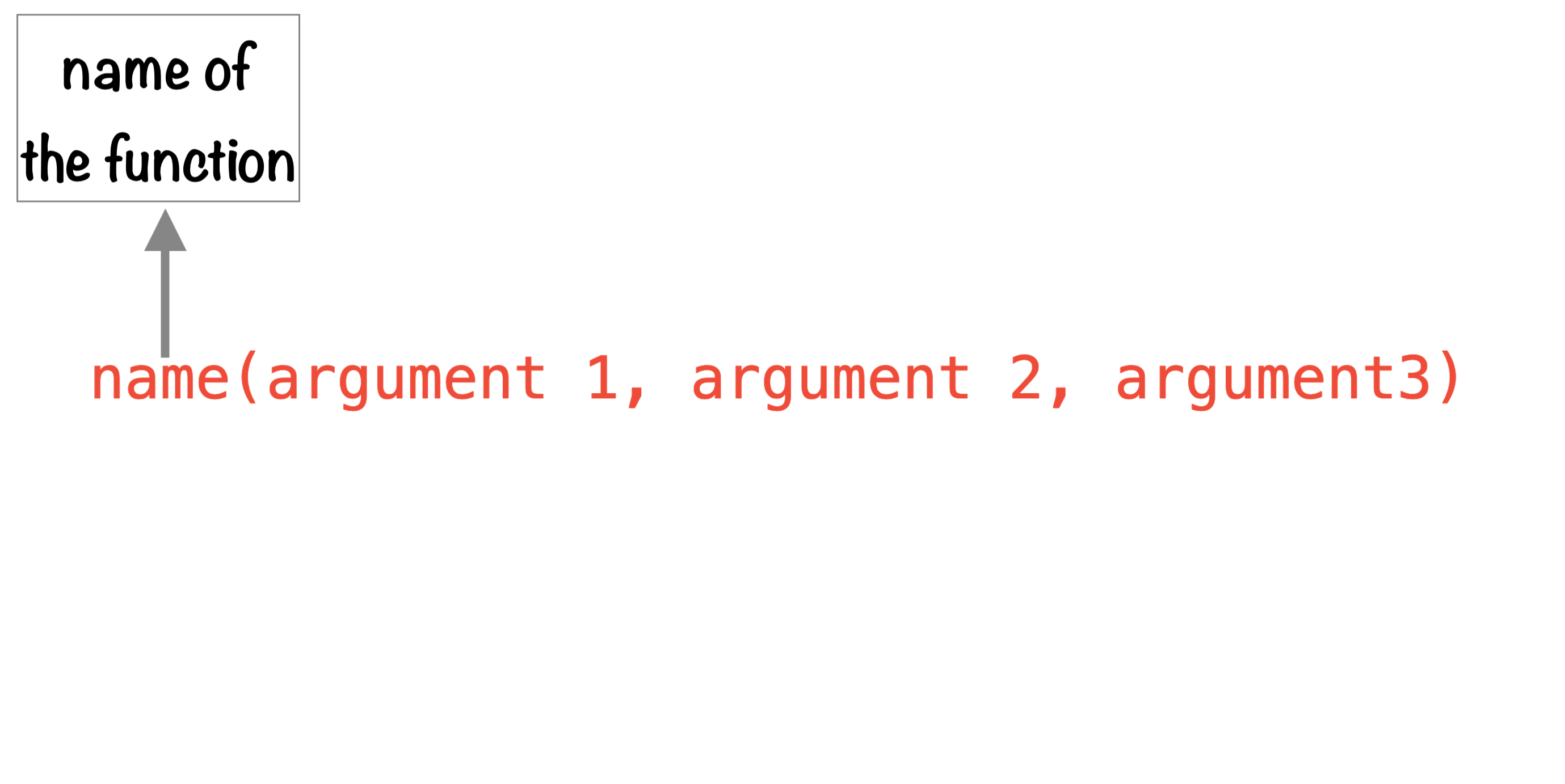
Structure of R Function
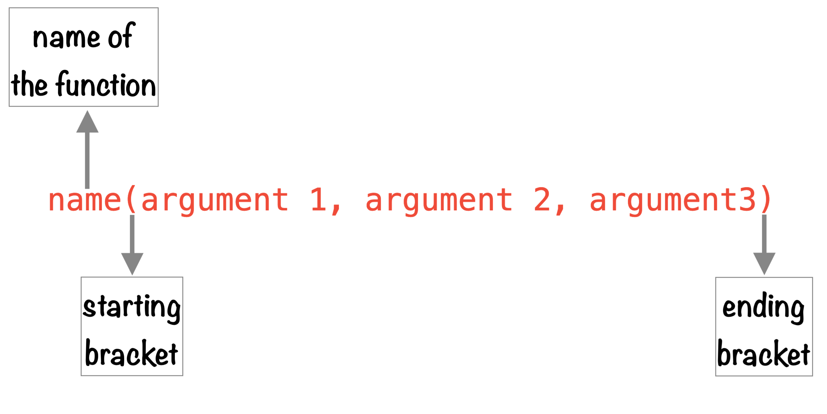
Structure of R Function
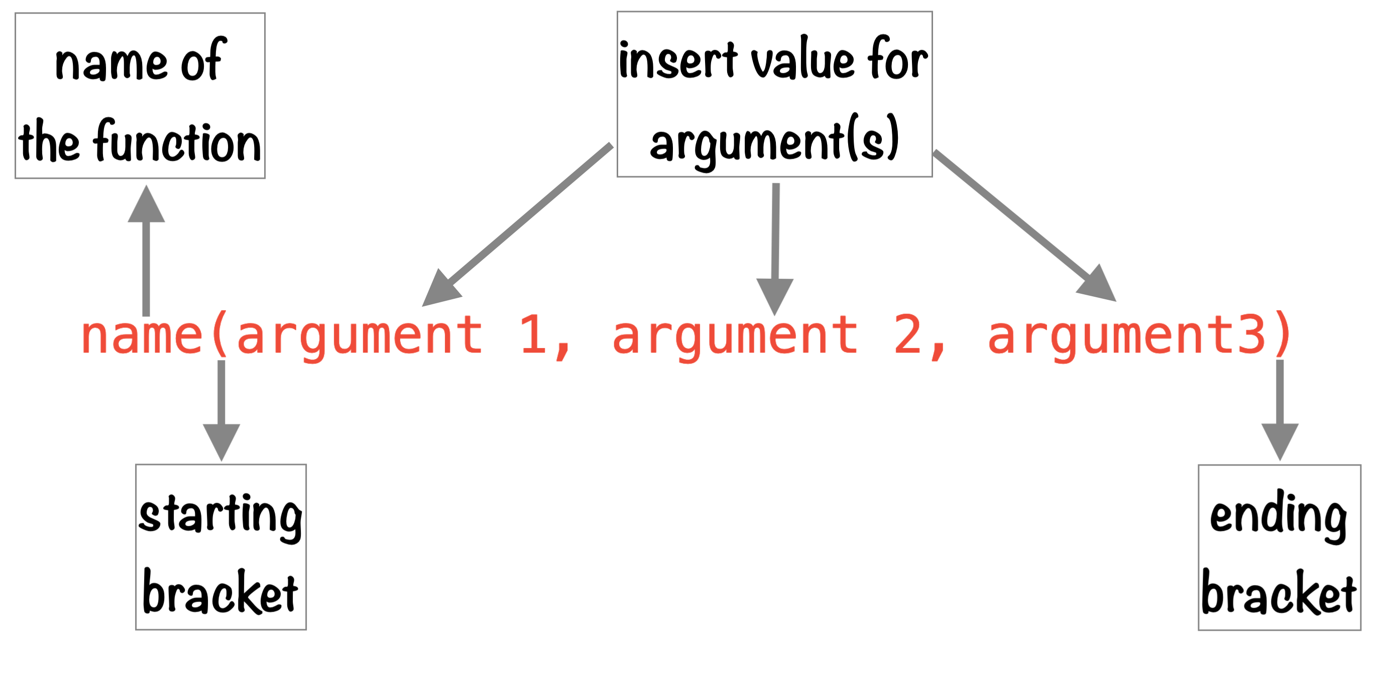
Structure of R Function

COMMENT
Artwork by Alision Horst
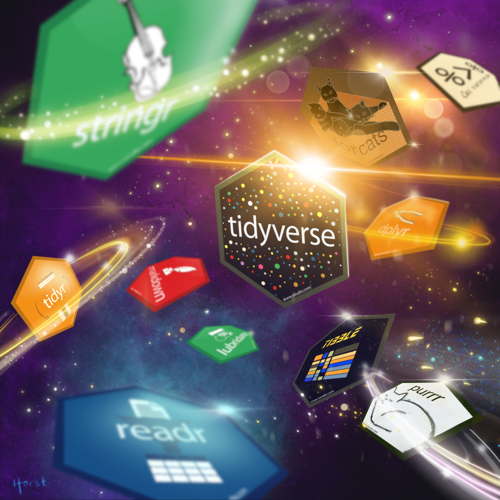
PACKAGES
R Packages
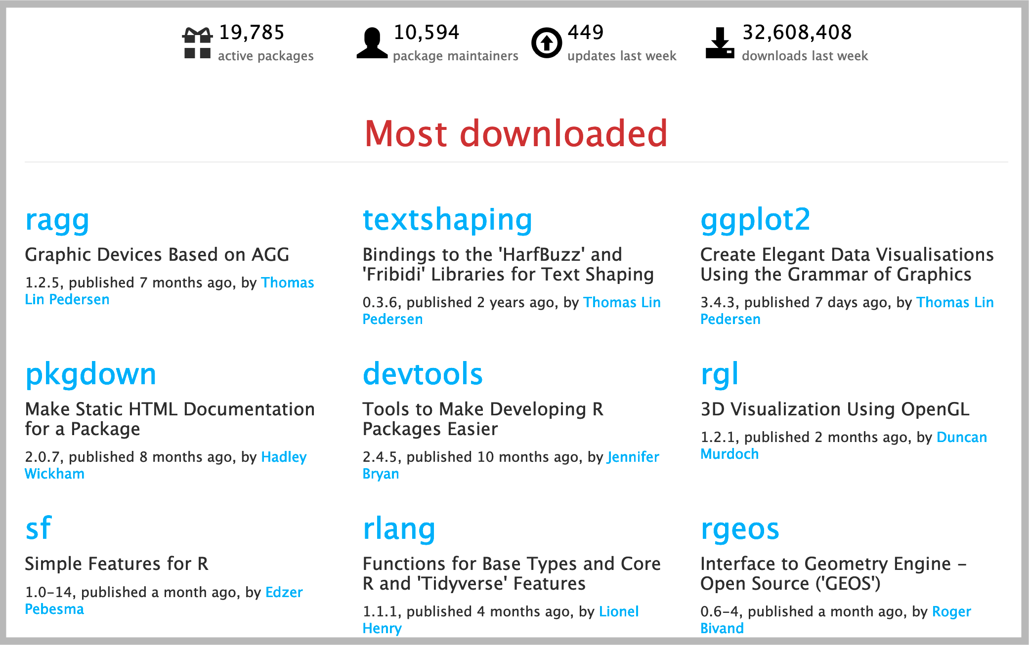
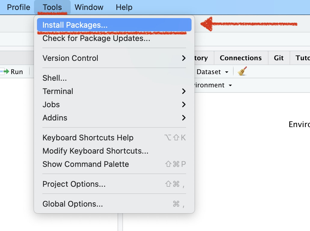
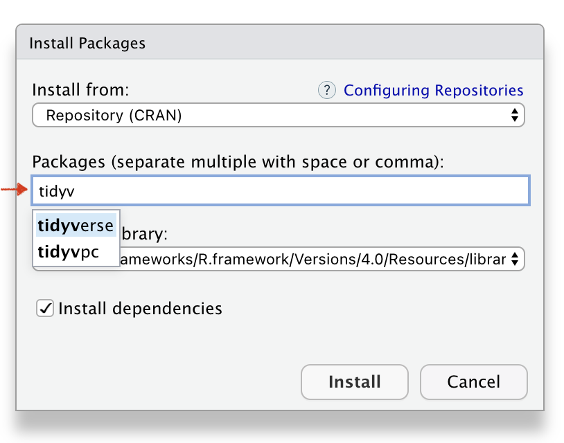
Install Packages
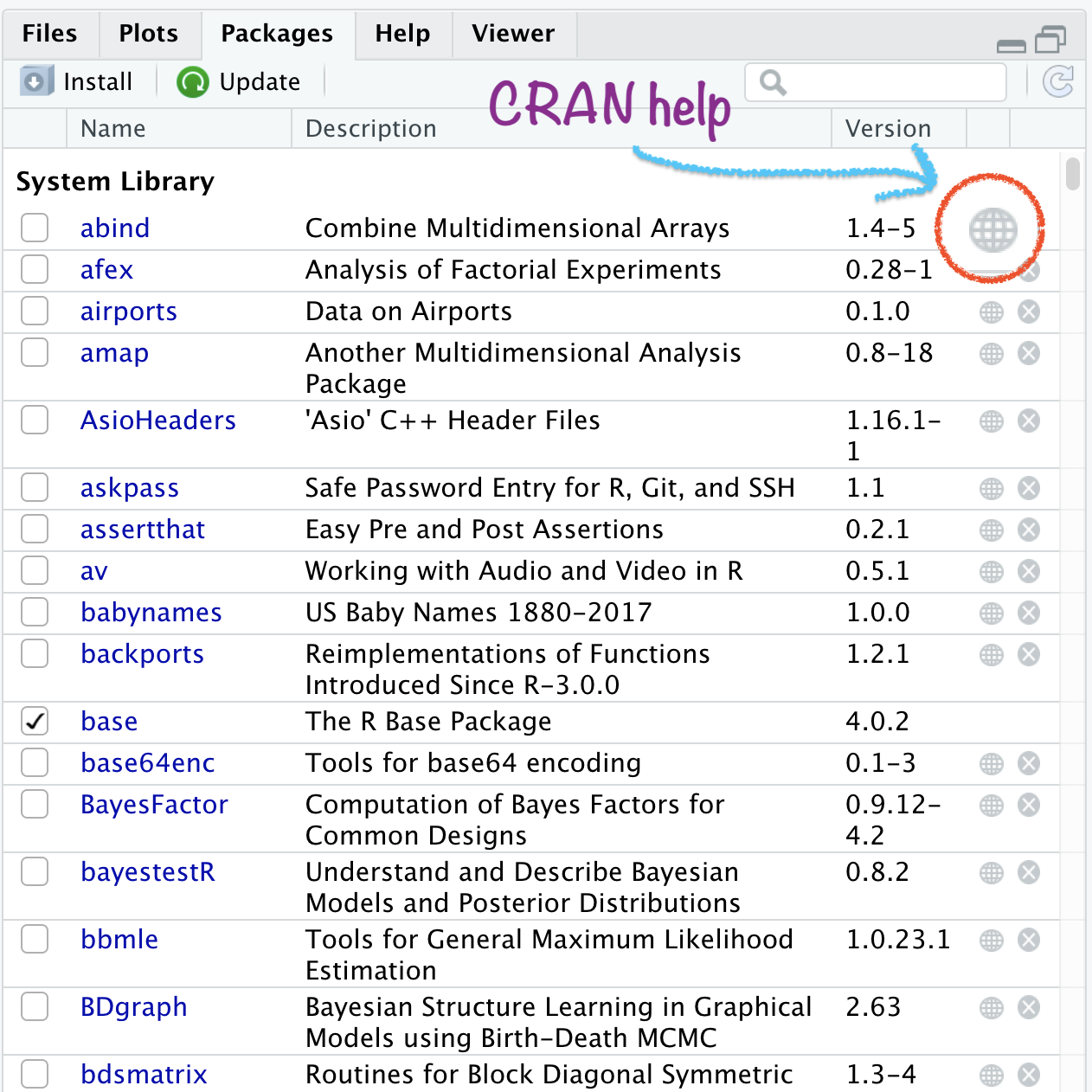
Name of the Packages
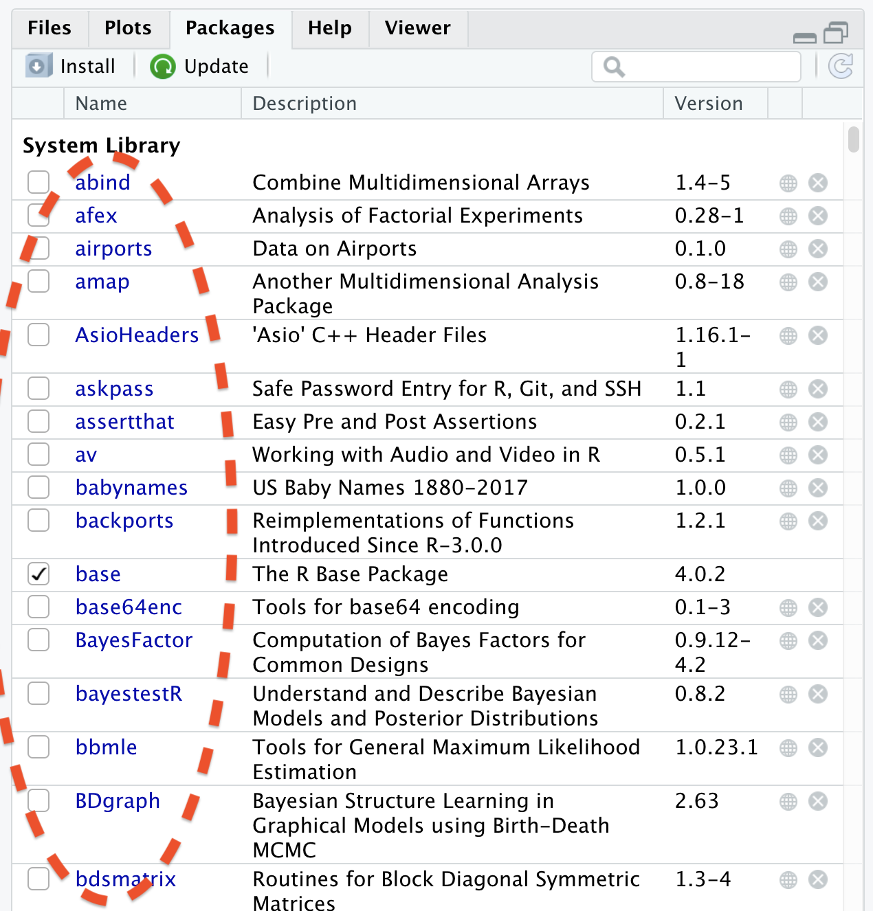
Installed Packages
Tools \(\rightarrow\) Package Updates
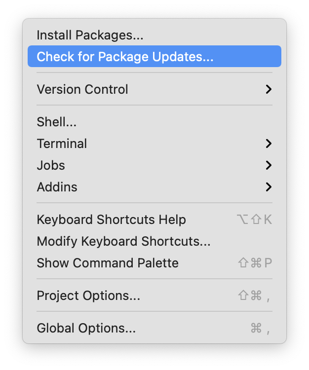
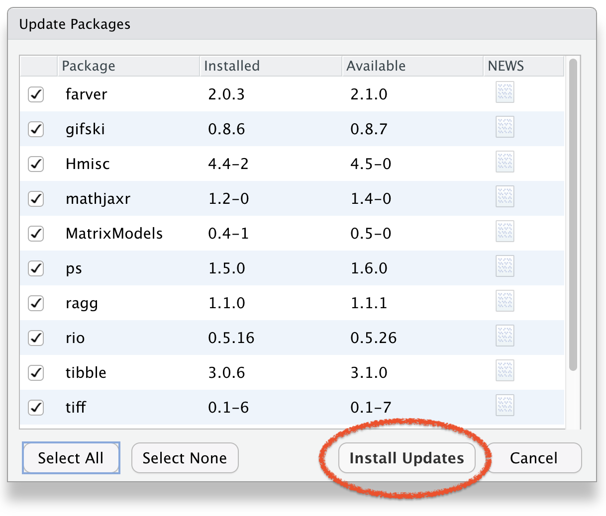
Select Packages to Update
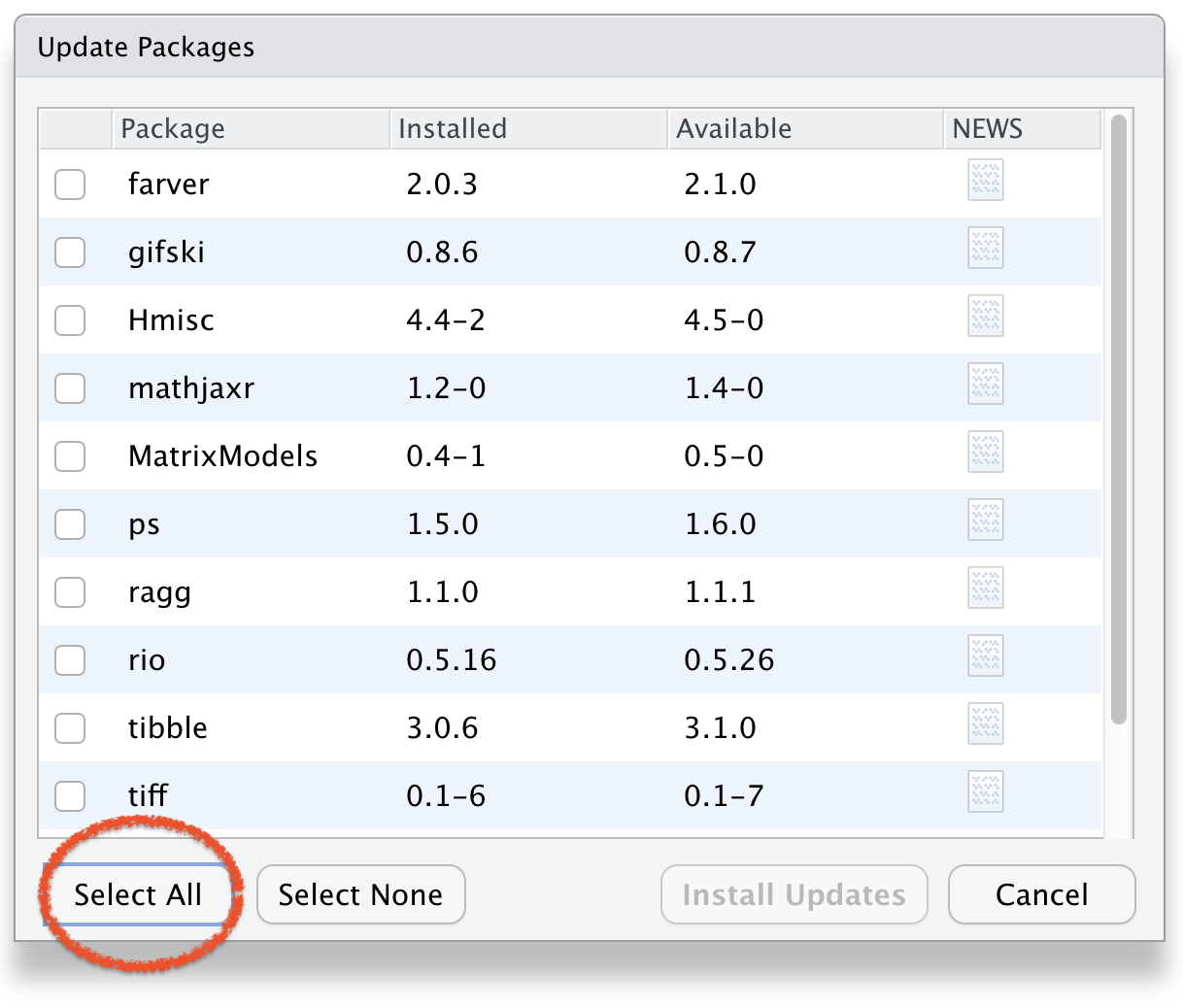
Click Install Updates
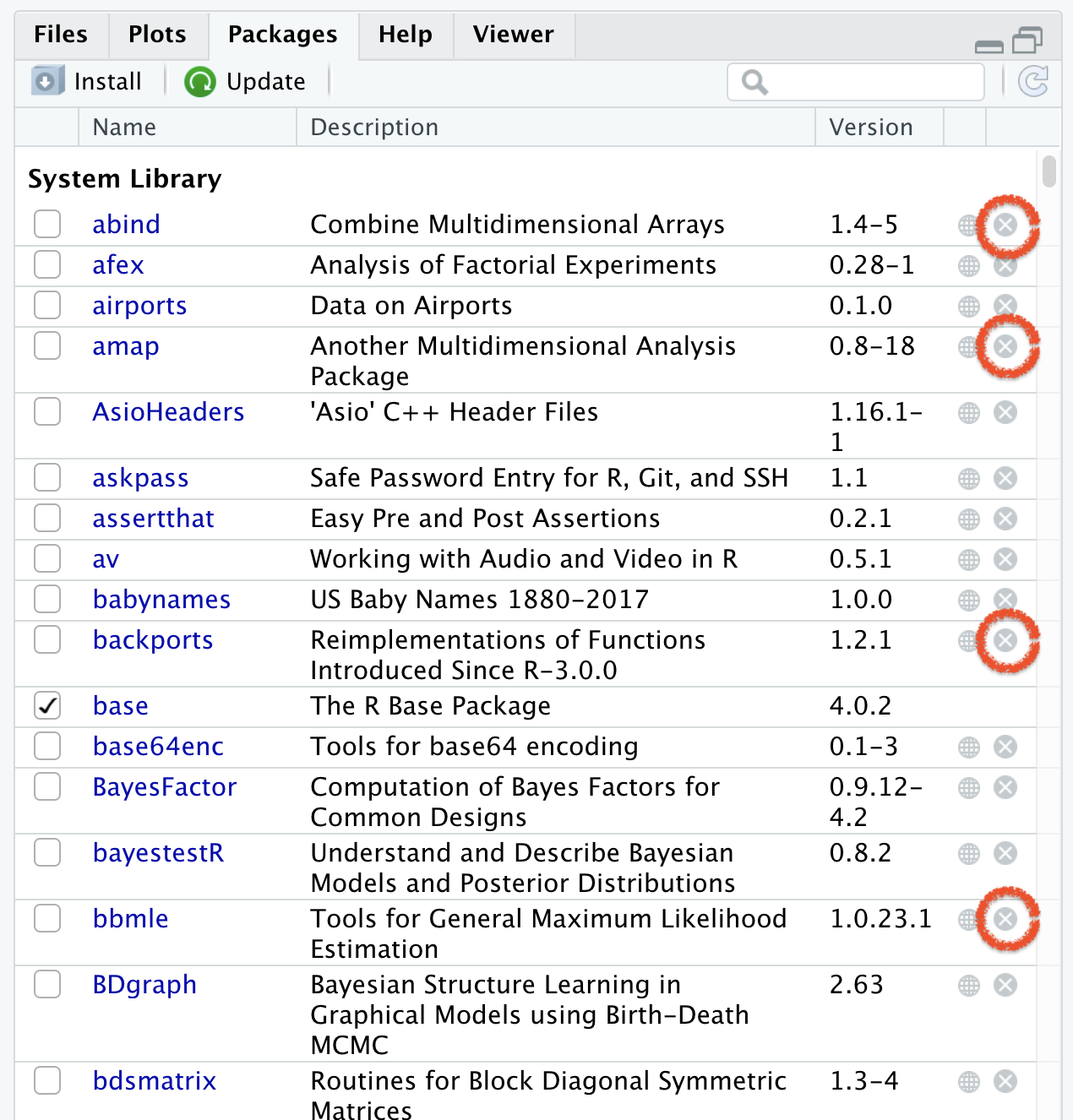
To Remove Packages

OBJECTS
Artwork by Alision Horst
RStudio Environment Window

🤔 How to combine all these objects and form a data set?

COMMUNITY
Artwork by Alision Horst
RStudio: Package Website
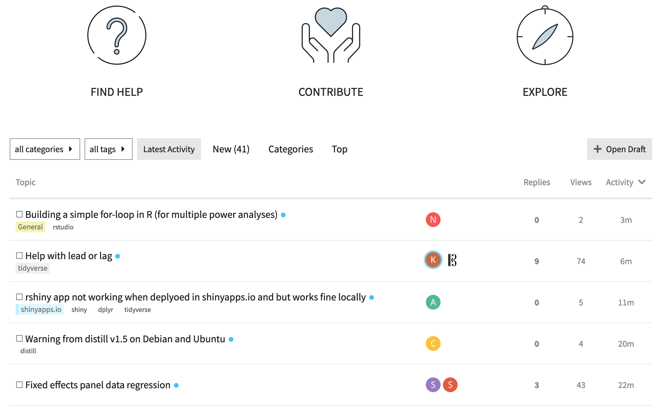
Posit Community
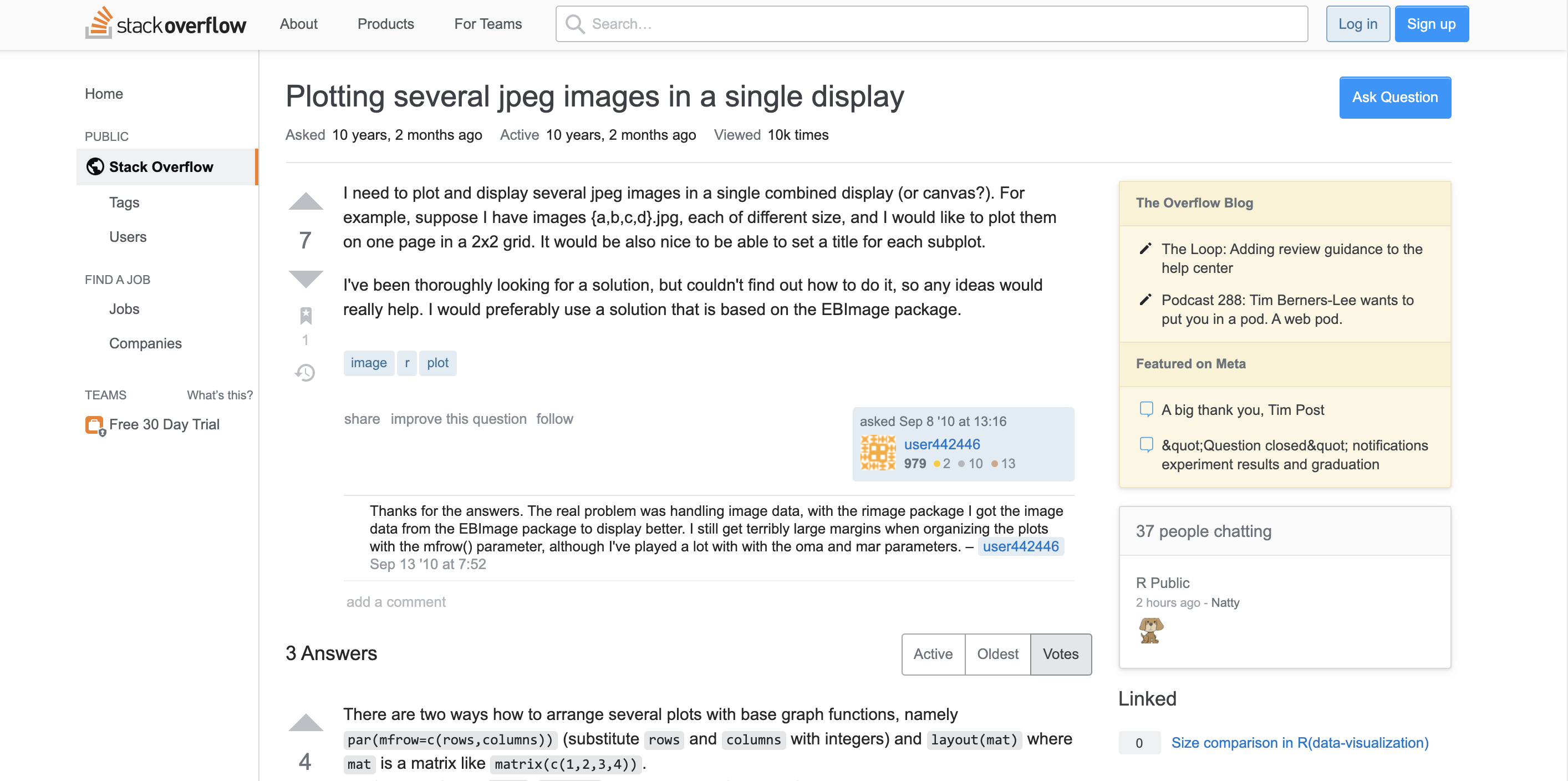
Stack Overflow
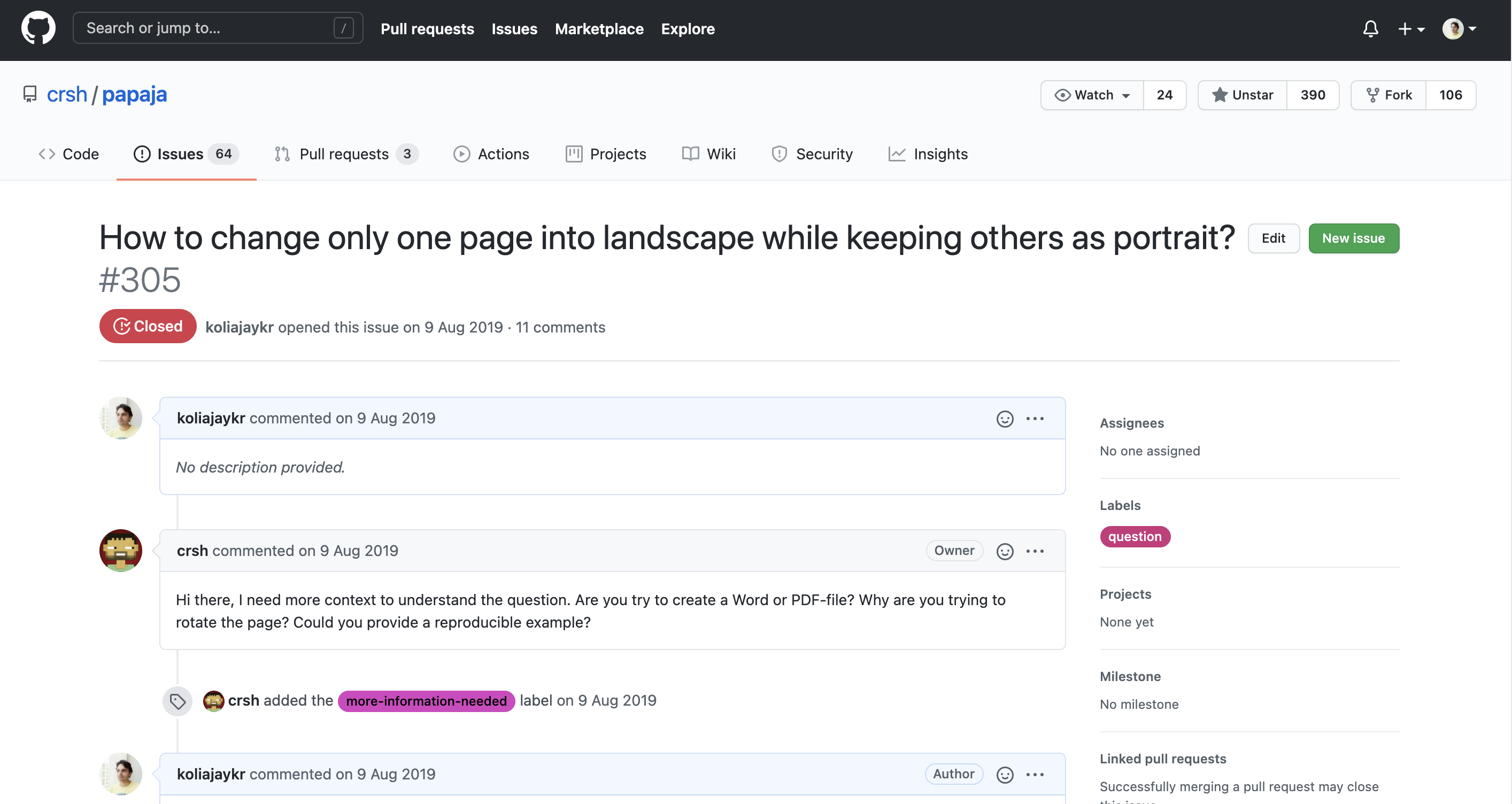
GitHub
QUARTO
Quarto is the Next Generation of R Markdown
![]()
![]()
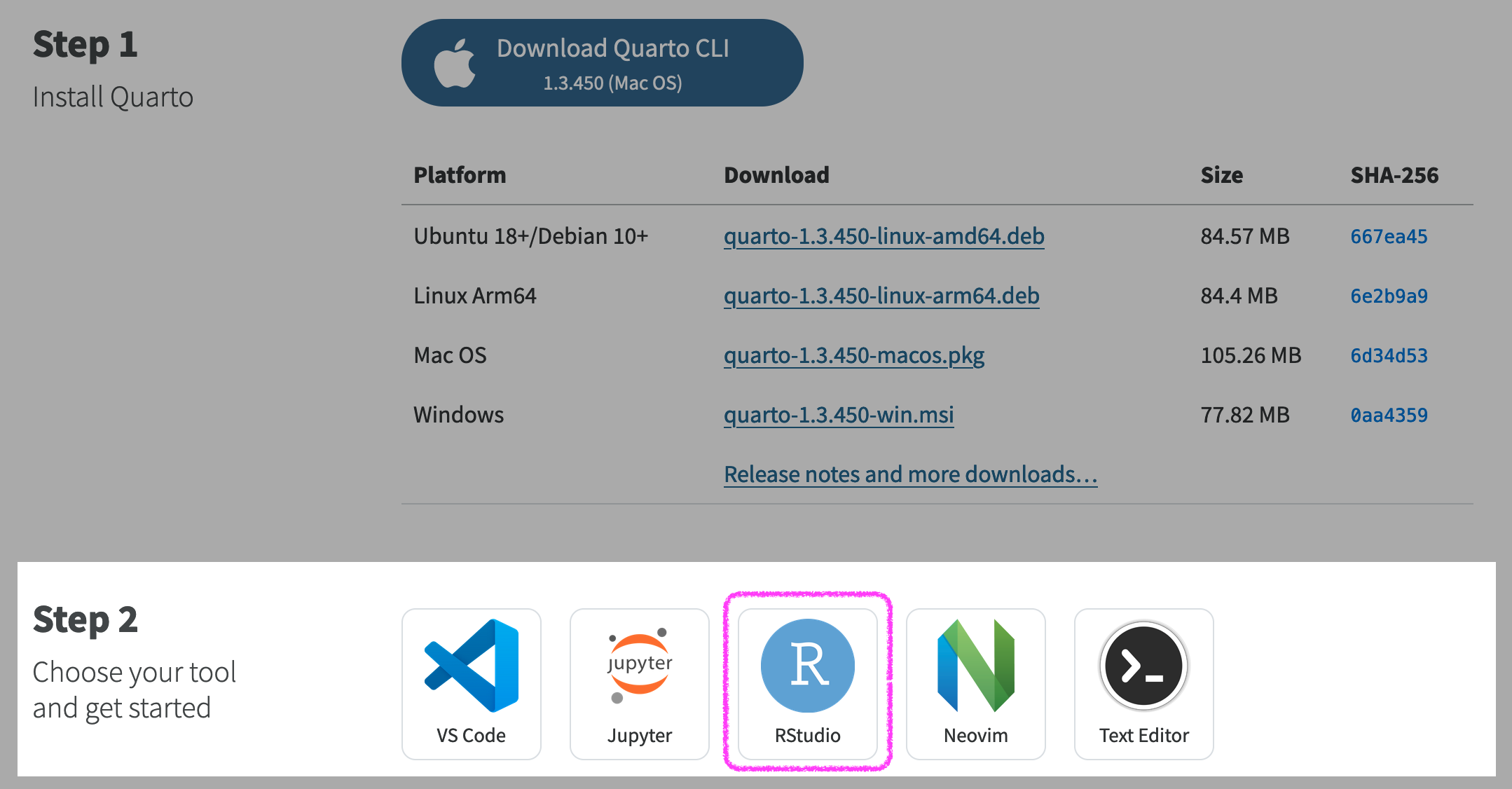
Download Quarto
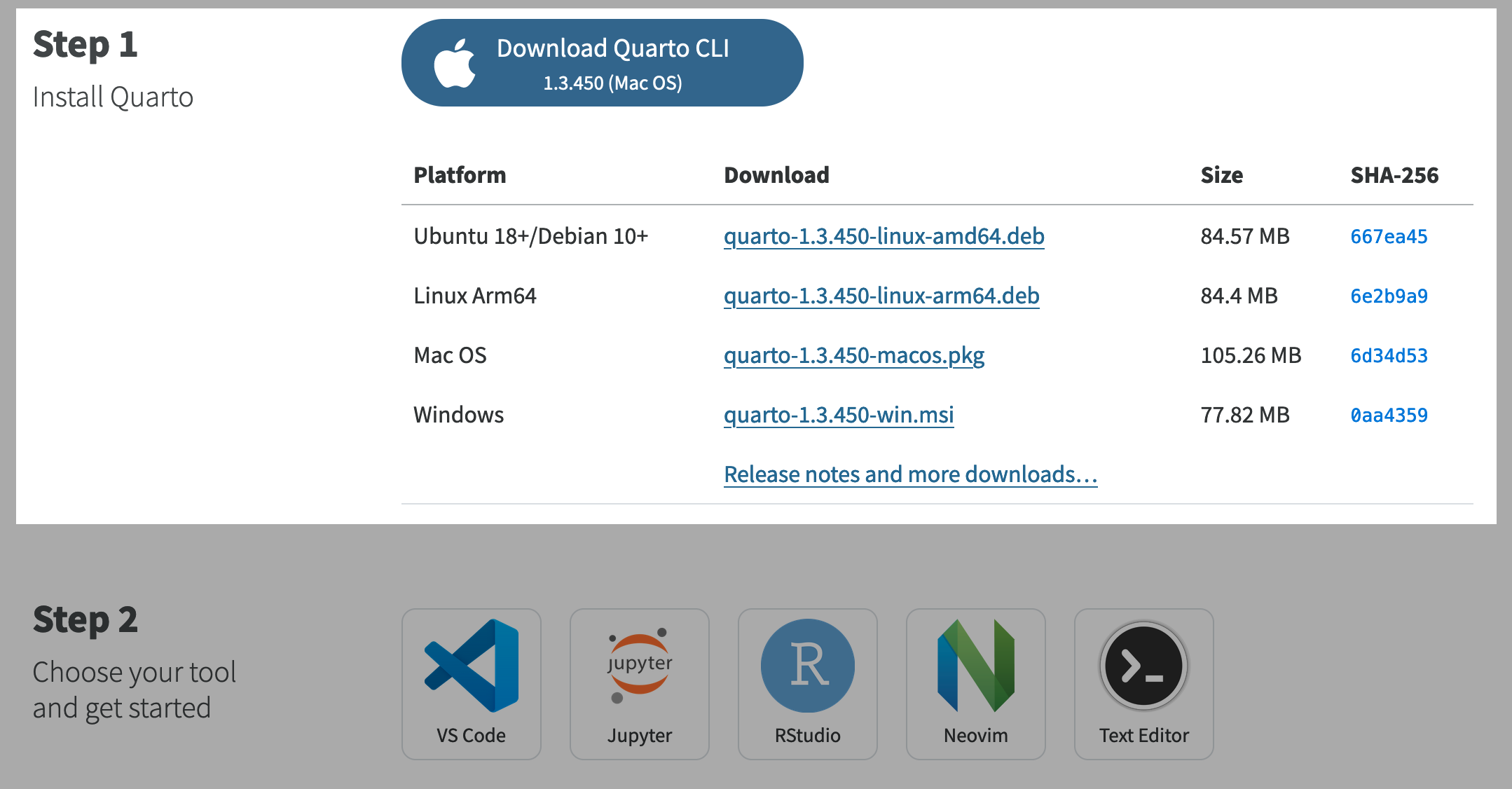
Get Started: Choose IDE
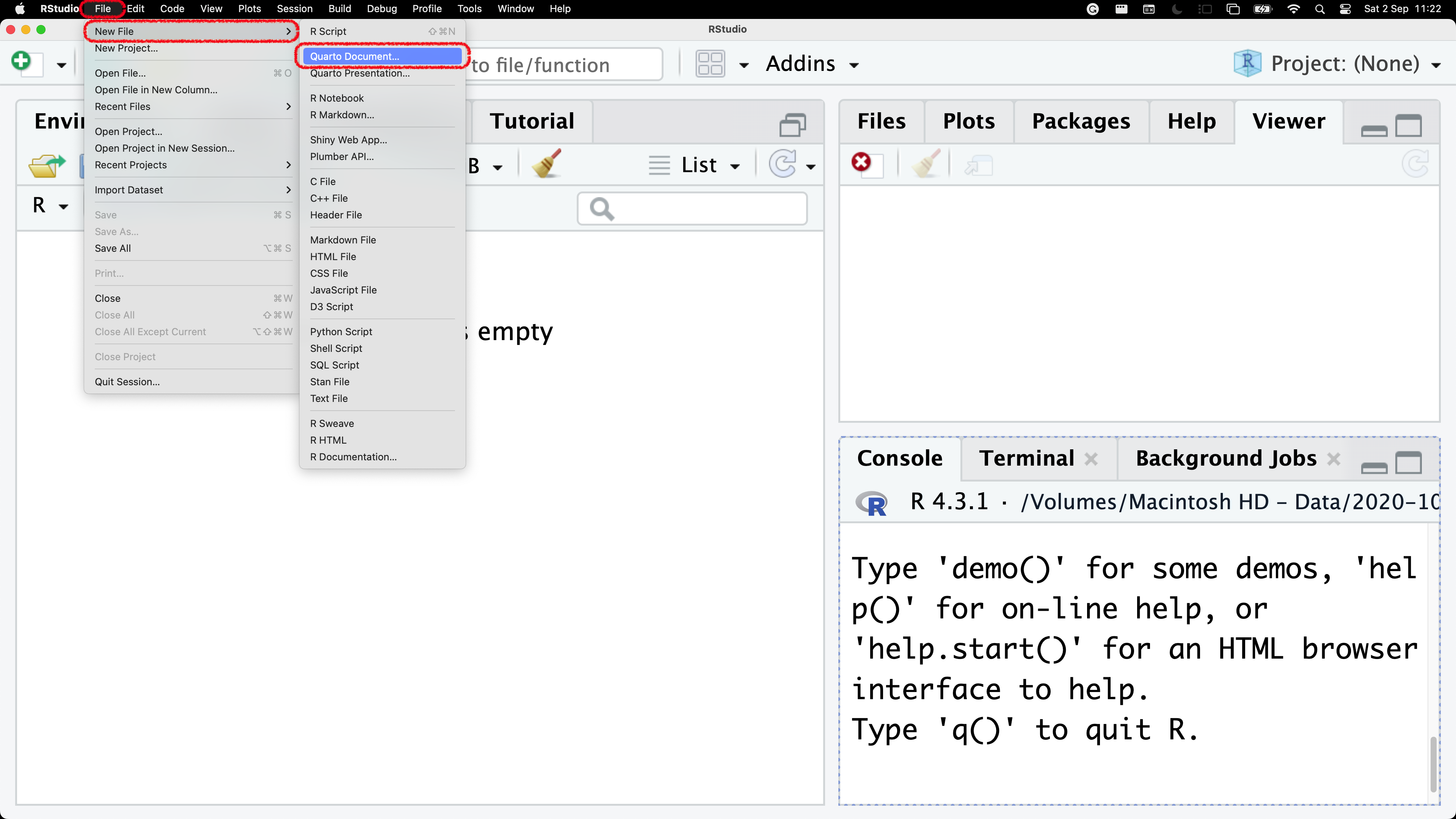
Create a New Quarto Document
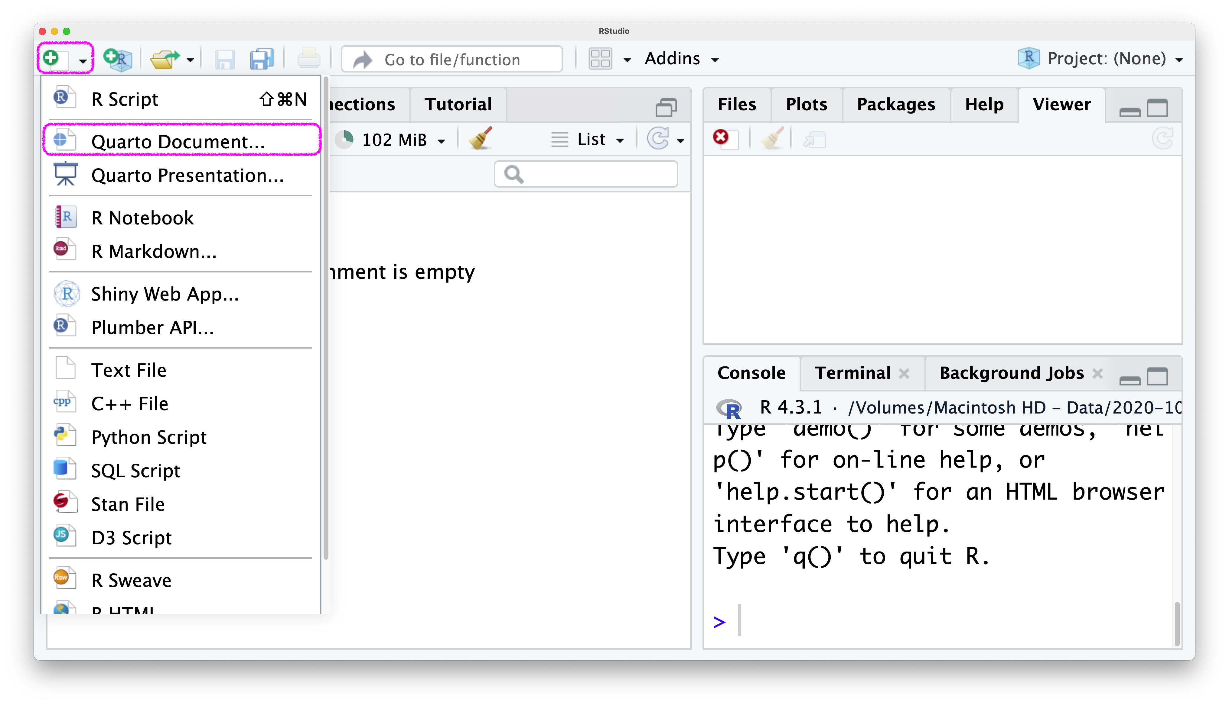
File \(\rightarrow\) New File \(\rightarrow\) Quarto Document
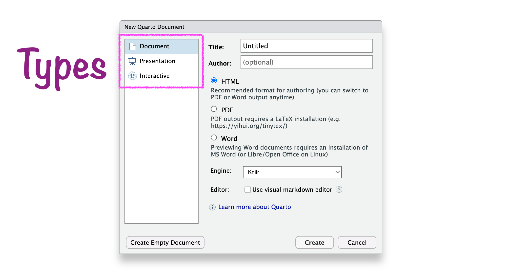
New Quarto Document

New Quarto Document
New Quarto Document

New Quarto Document
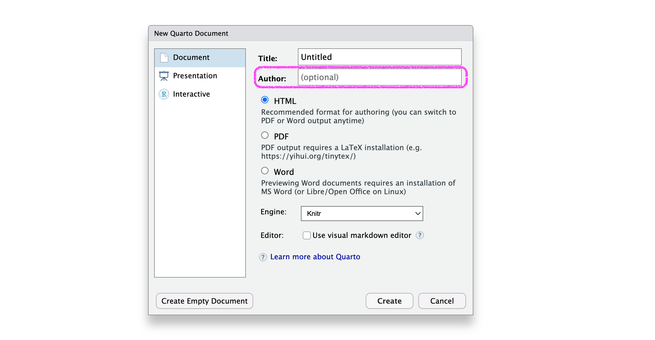
New Quarto Document
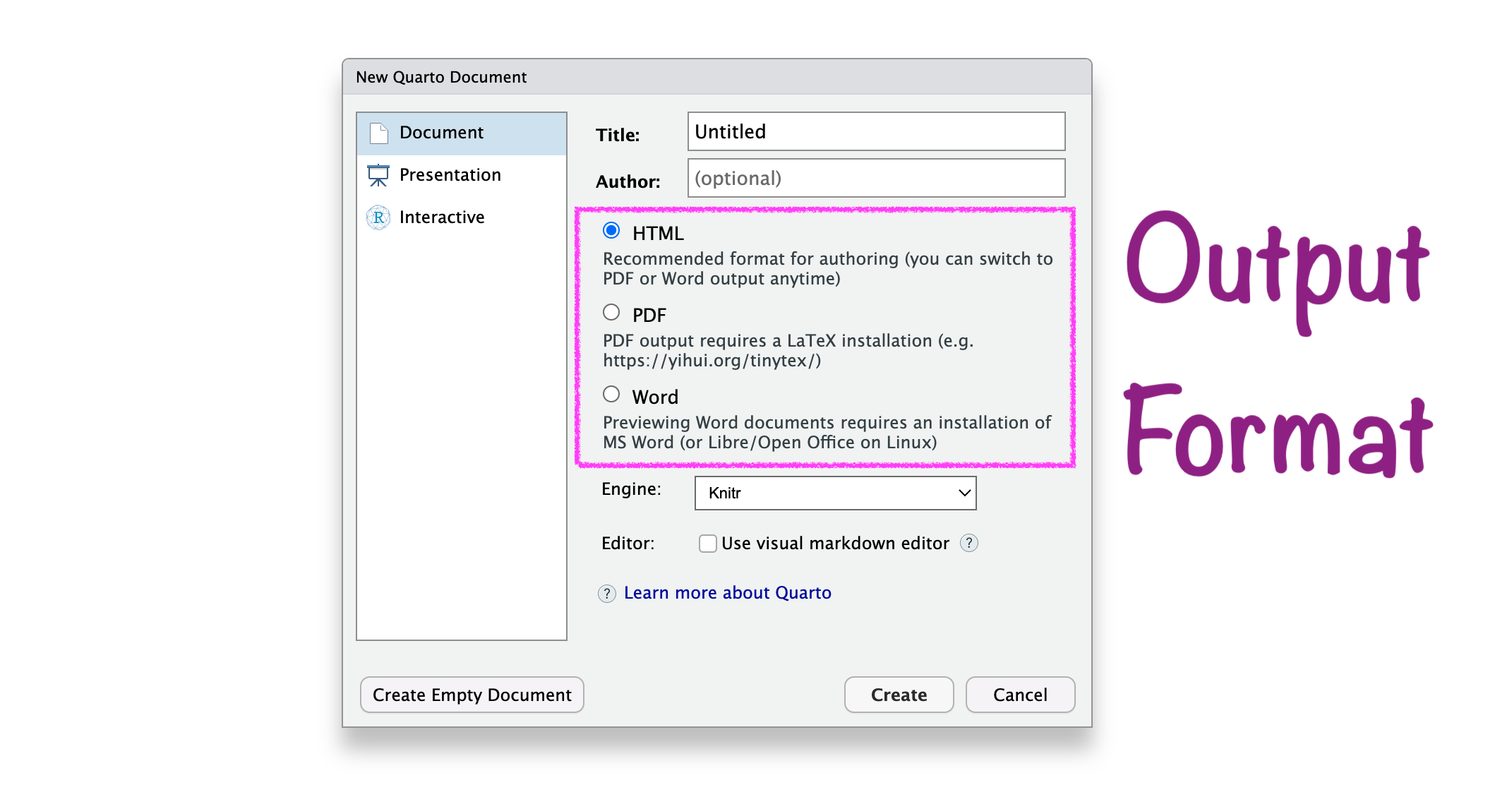
New Quarto Document

New Quarto Document

New Quarto Document
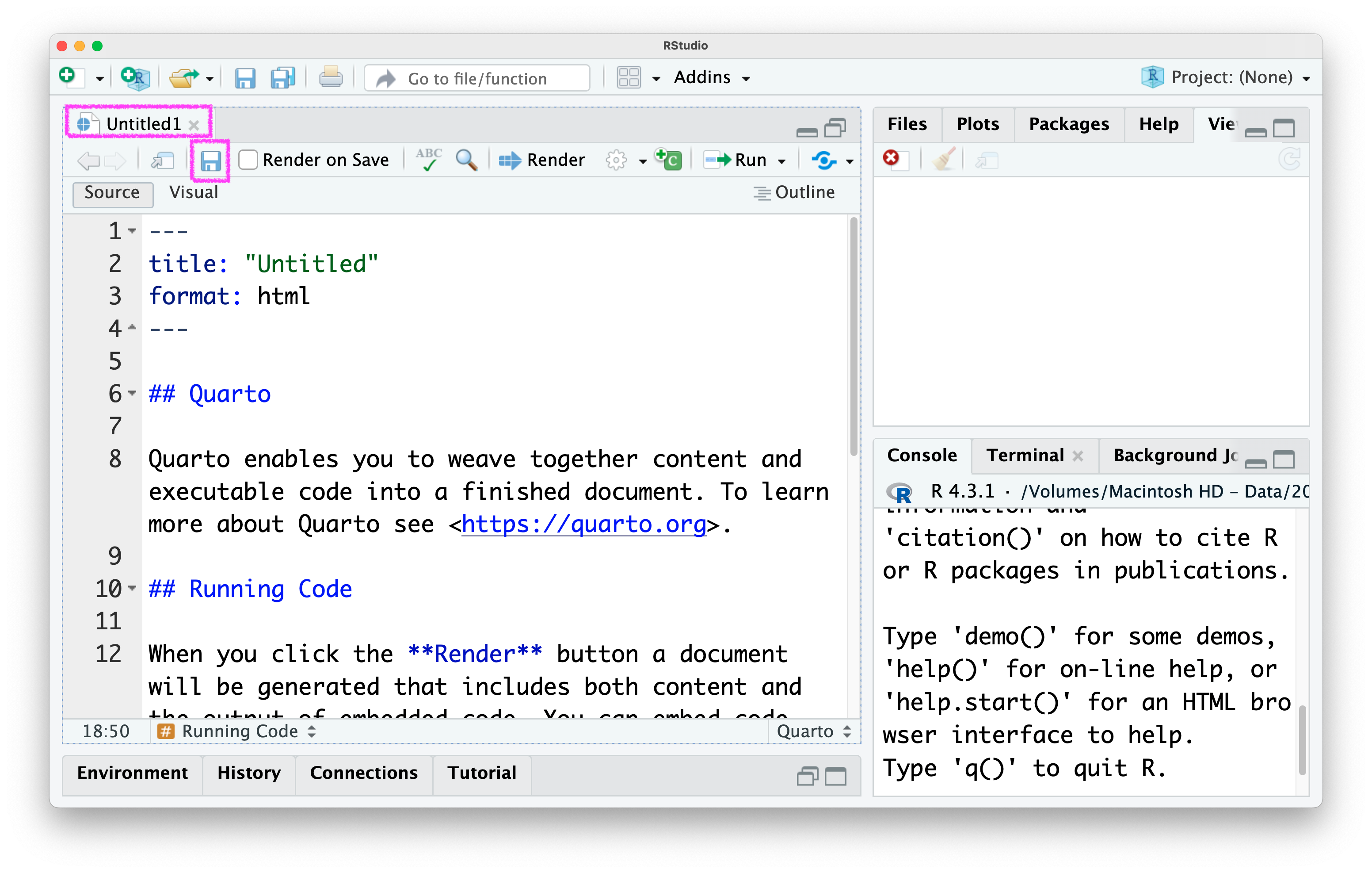
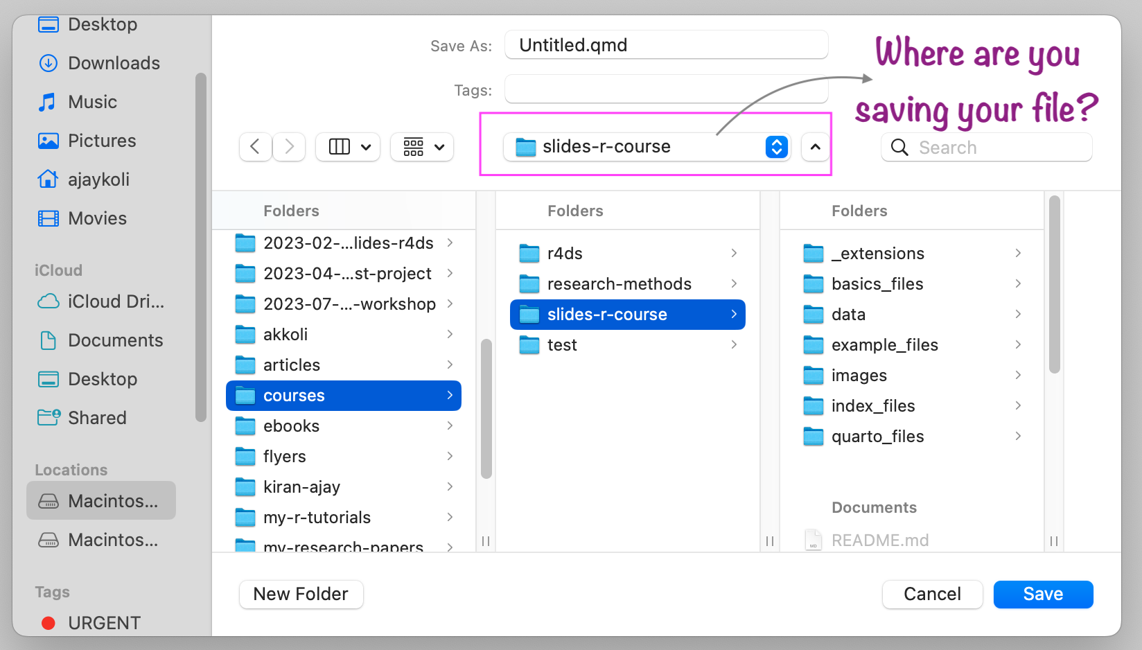
Save Quarto Document
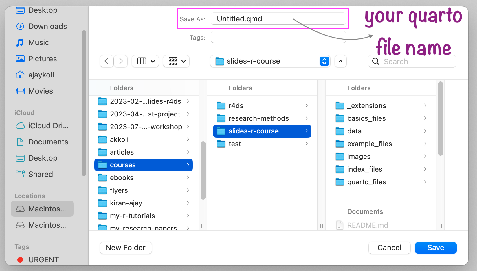
Save Quarto Document
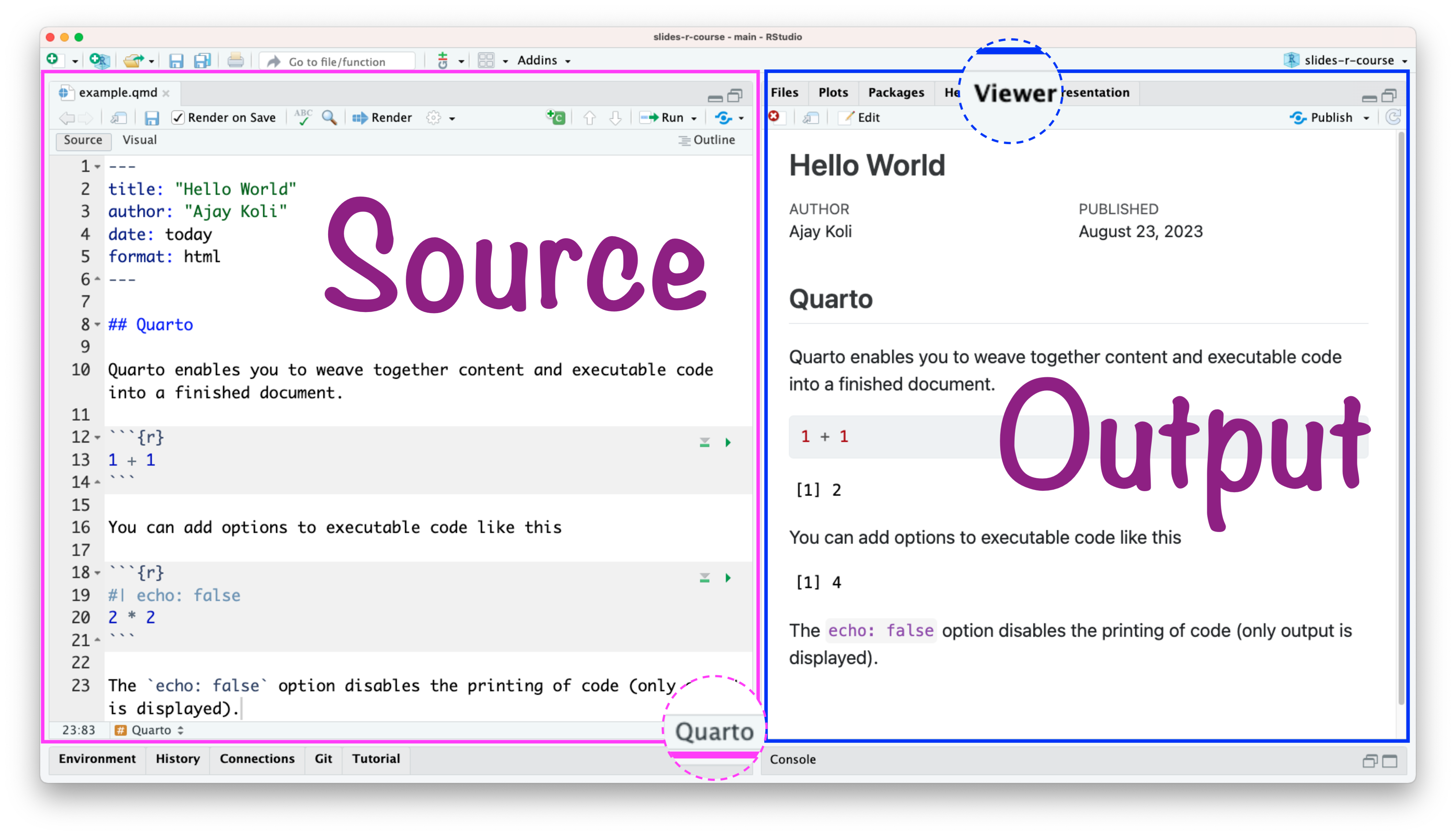
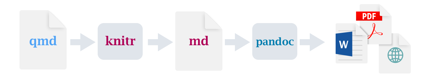
Process When You Render the Quarto Document
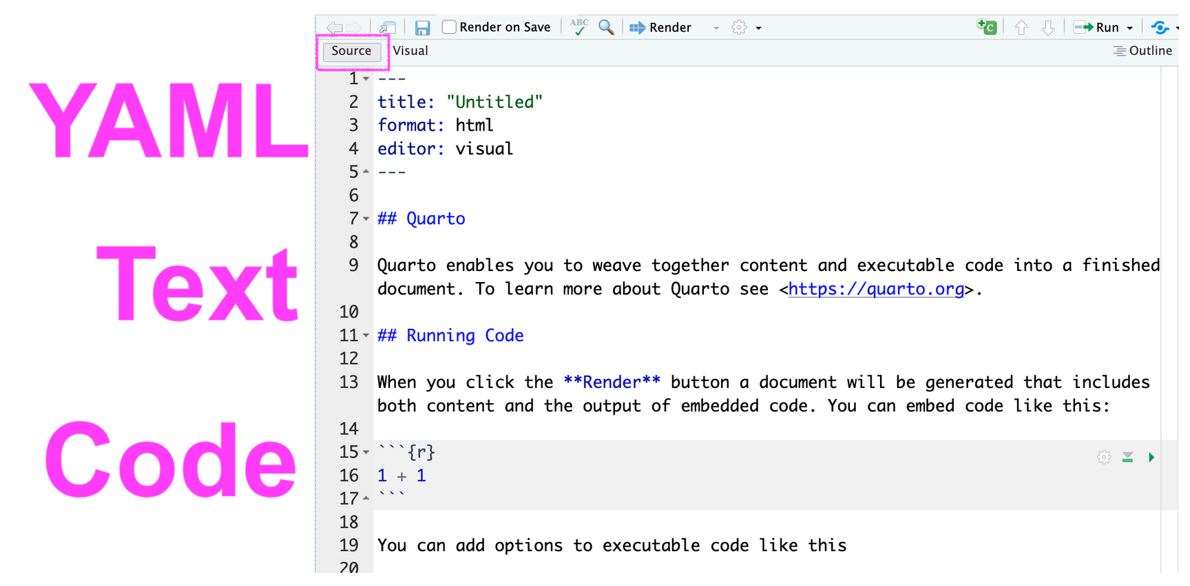
Source Editor vs. Visual Editor
Visual Editor

Visual Editor
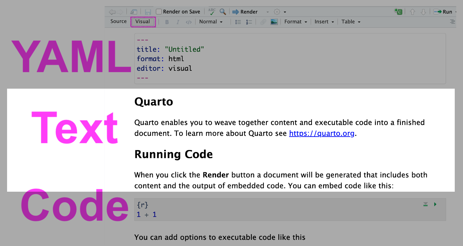
Visual Editor
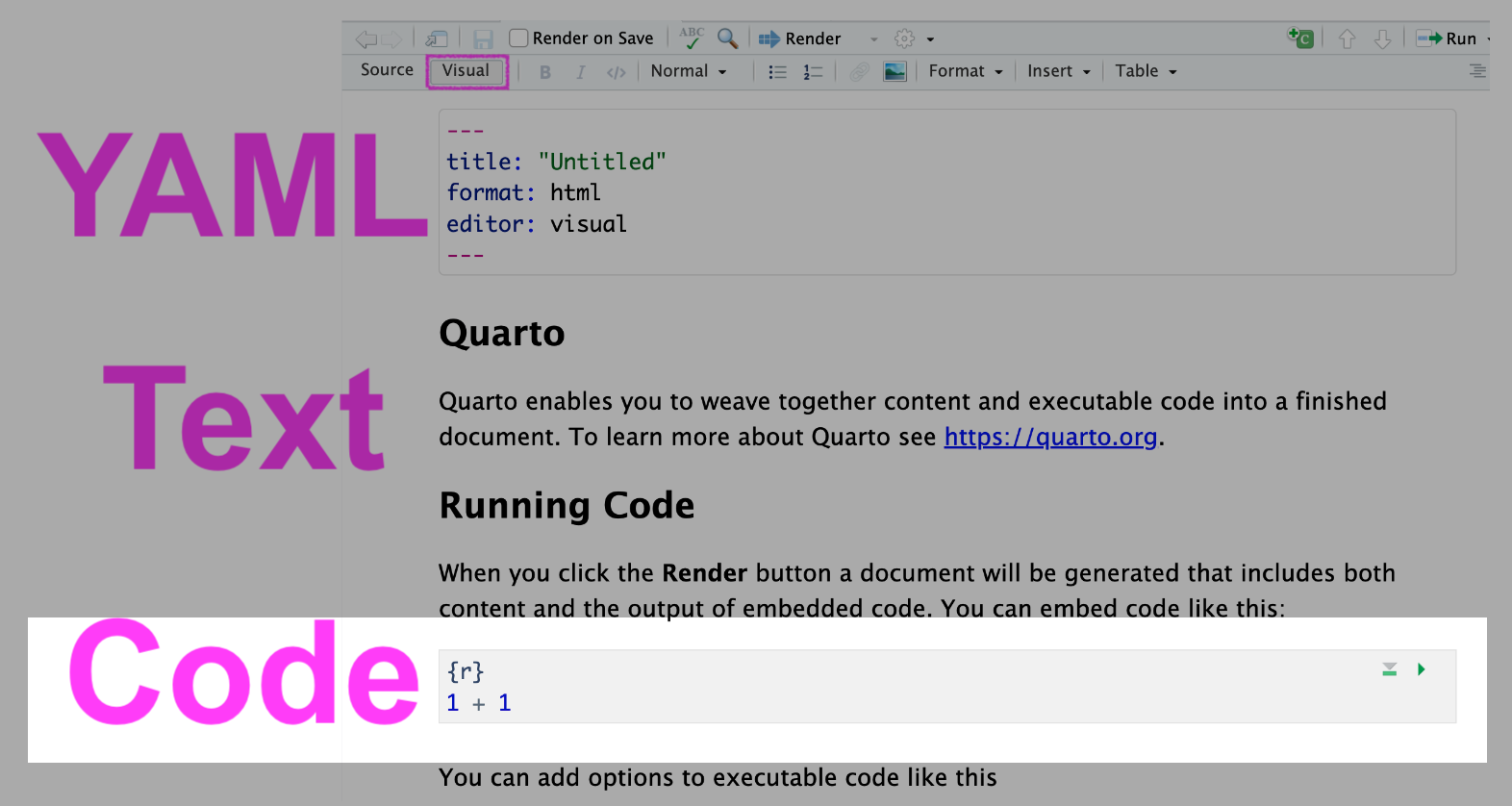
Source Editor
MARKDOWN
Add Images
If image is saved in your computer,

| Markdown Syntax | Output |
|---|---|
|
 |
Add Images
If image is taken from the internet,


Know Your Data
Data: Variables
     name income age place weight_kg
1    Bhim  23000  23    MH        50
2    Rama  25000  25    RJ        52
3    Sara  16000  16    DL        61
4   Phule   4000  40    HR        40
5 Savitri  34000  34    HR        70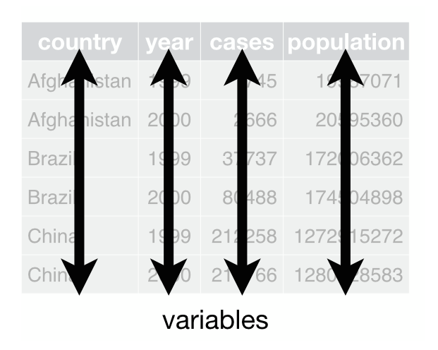
Data: Observations
     name income age place weight_kg
1    Bhim  23000  23    MH        50
2    Rama  25000  25    RJ        52
3    Sara  16000  16    DL        61
4   Phule   4000  40    HR        40
5 Savitri  34000  34    HR        70
Data: Values
     name income age place weight_kg
1    Bhim  23000  23    MH        50
2    Rama  25000  25    RJ        52
3    Sara  16000  16    DL        61
4   Phule   4000  40    HR        40
5 Savitri  34000  34    HR        70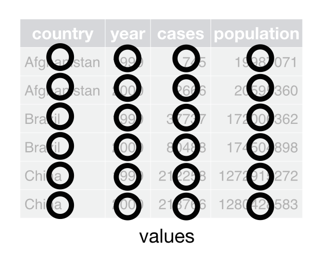
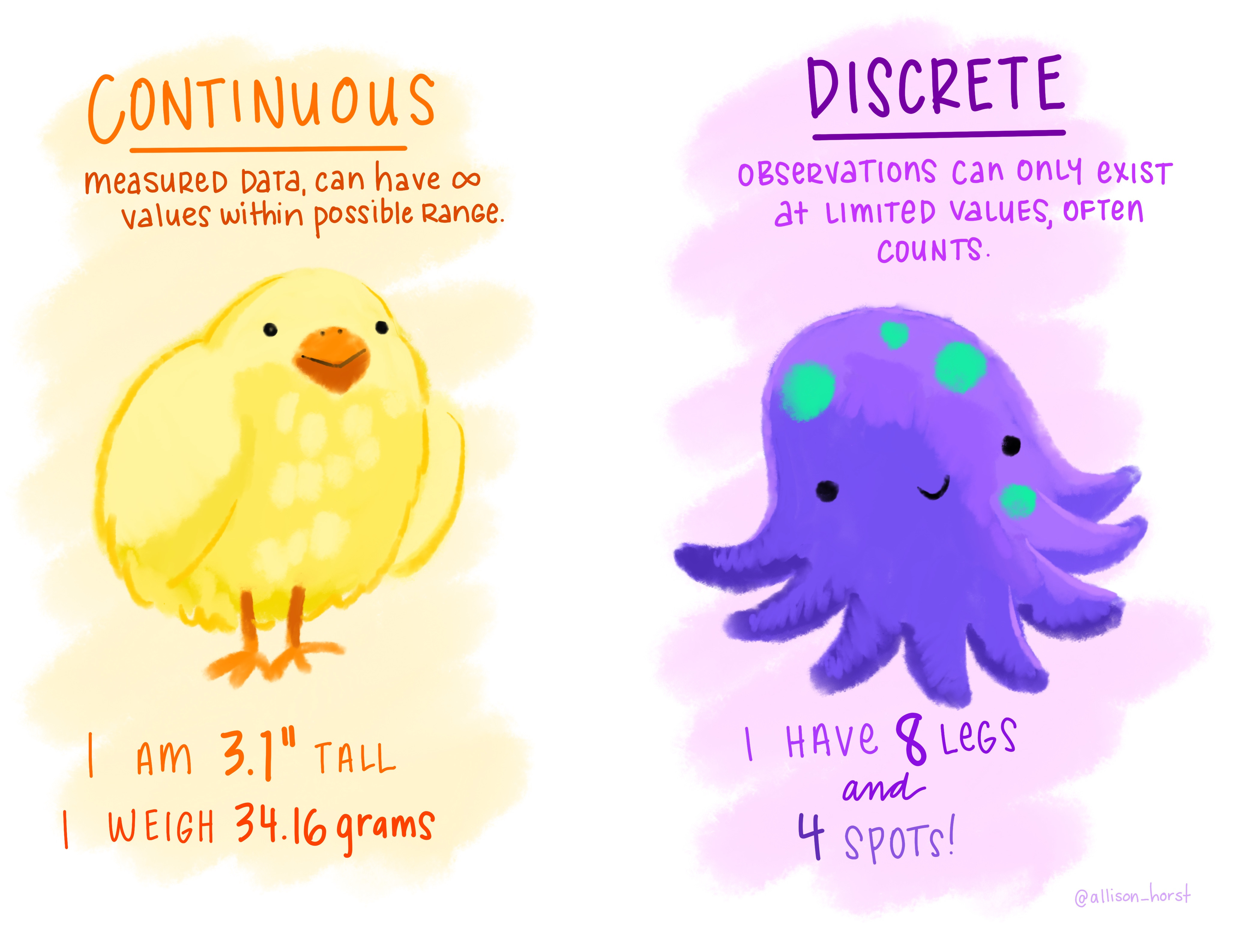
Numeric Value Types
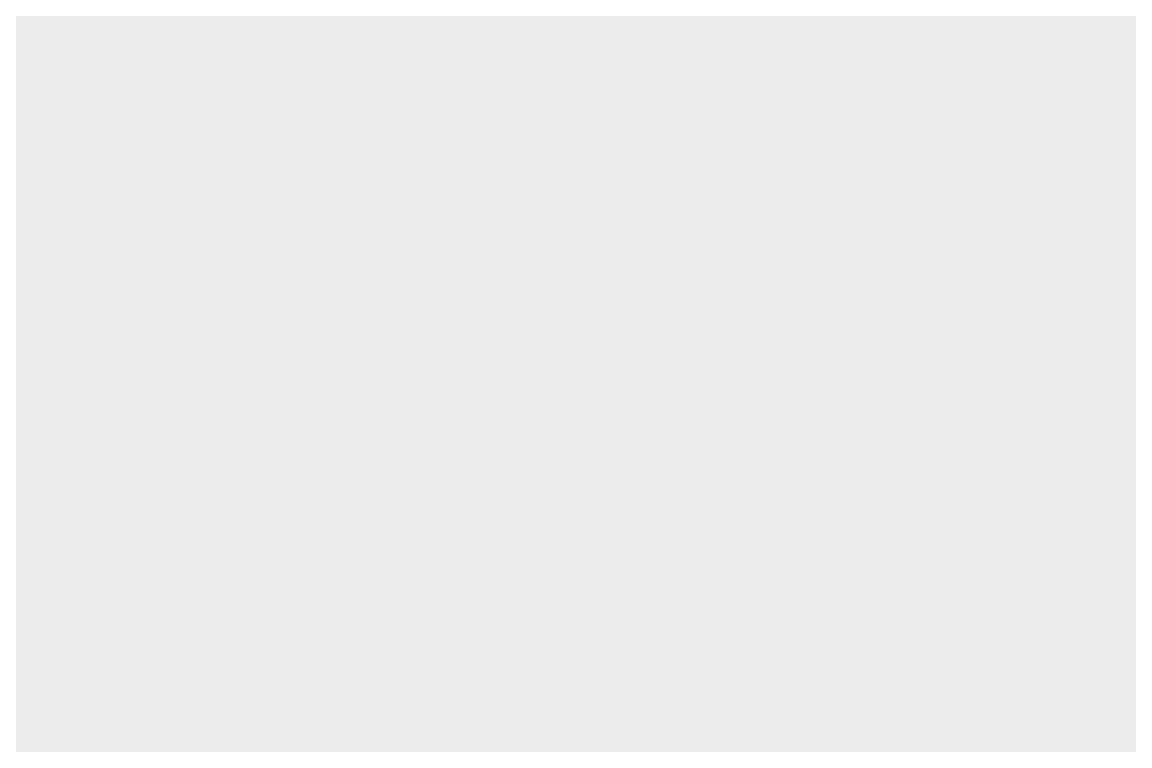
palmerpenguins
R package name palmerpenguins & dataset name is penguins more information here.


Goal
How to visualize data using R package ggplot2.
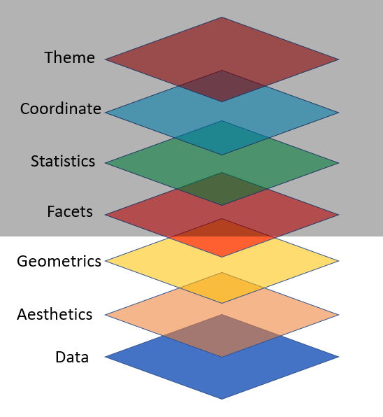
ggplot2 Layers
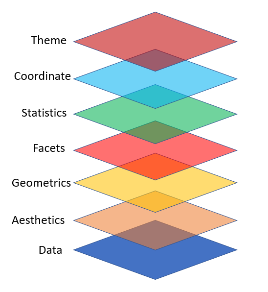
Import Data
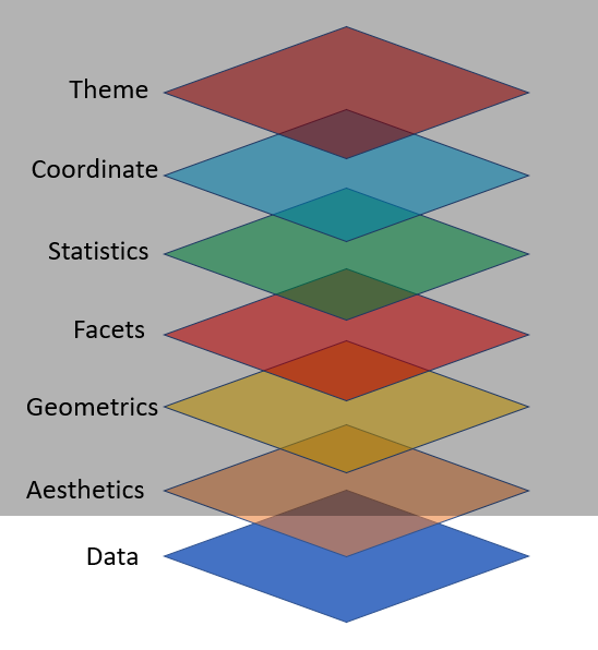

Map Variables Aesthetics
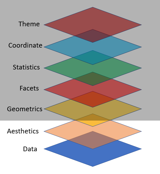
Add Geometric Shapes
🧠 YOUR TURN
05:00
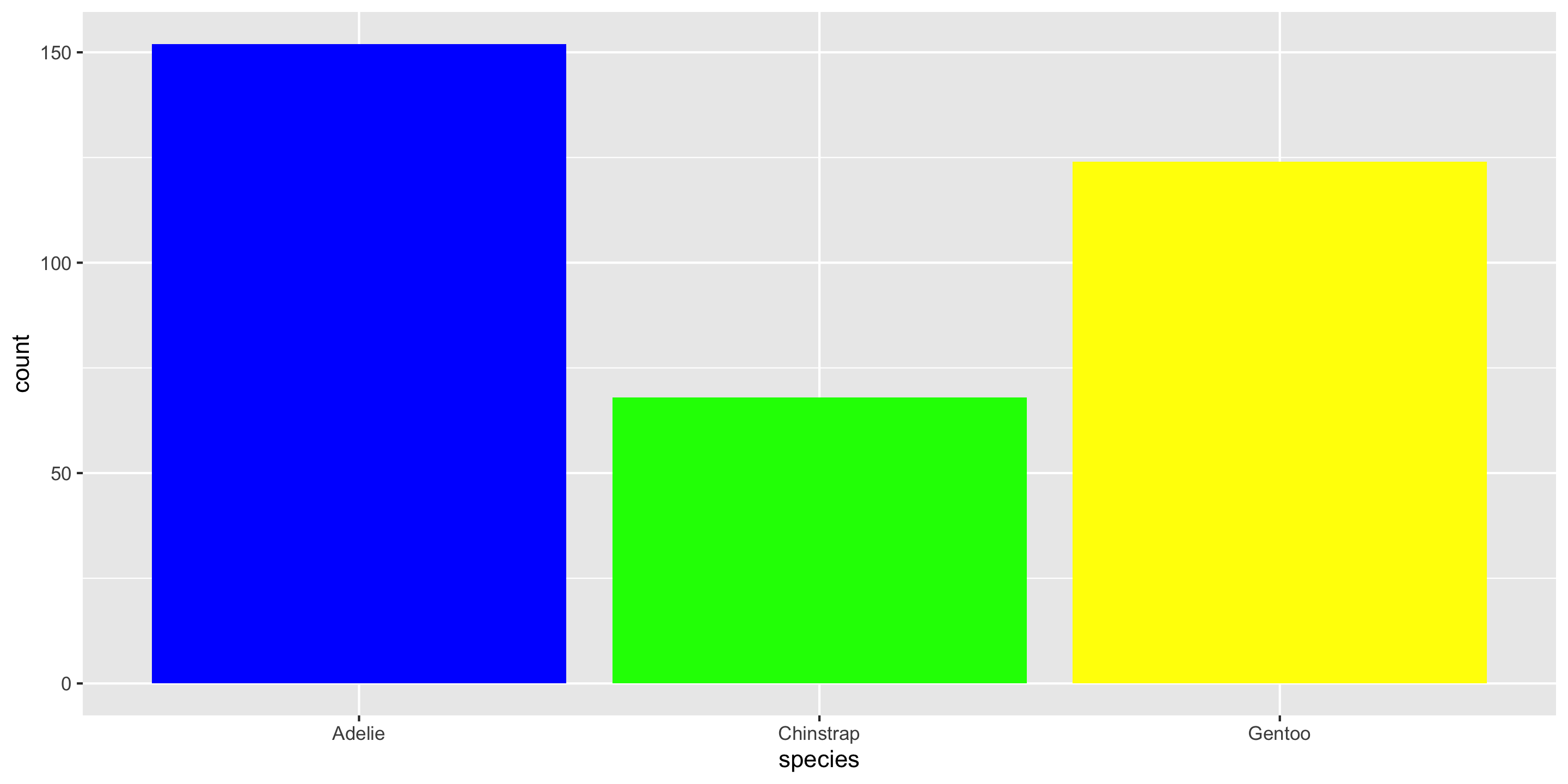
“Fill” Color

“Fill” Colors
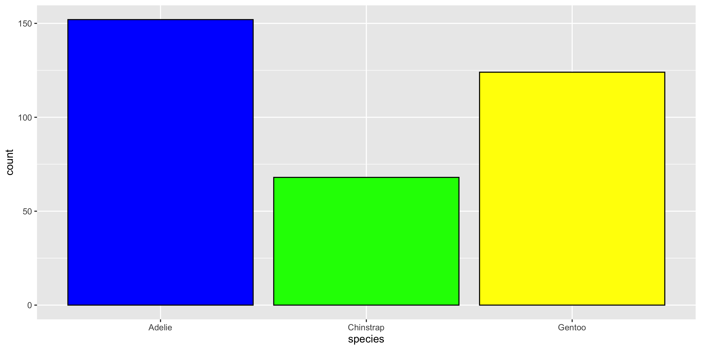
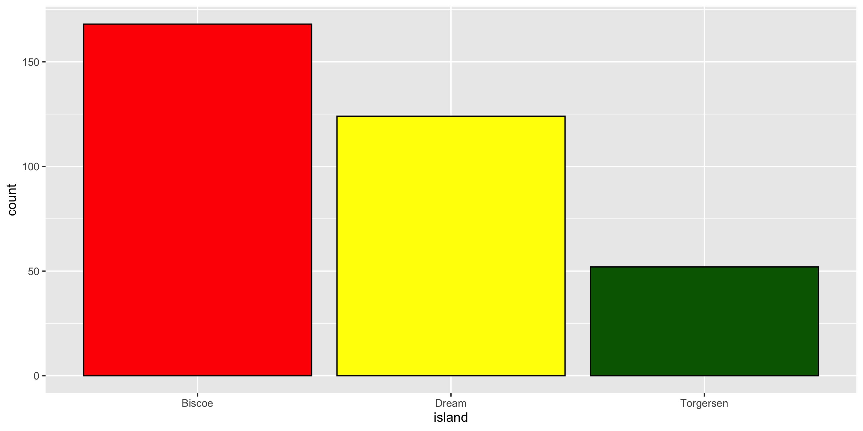
“Fill” & “Color” Colors
🧠 YOUR TURN
05:00
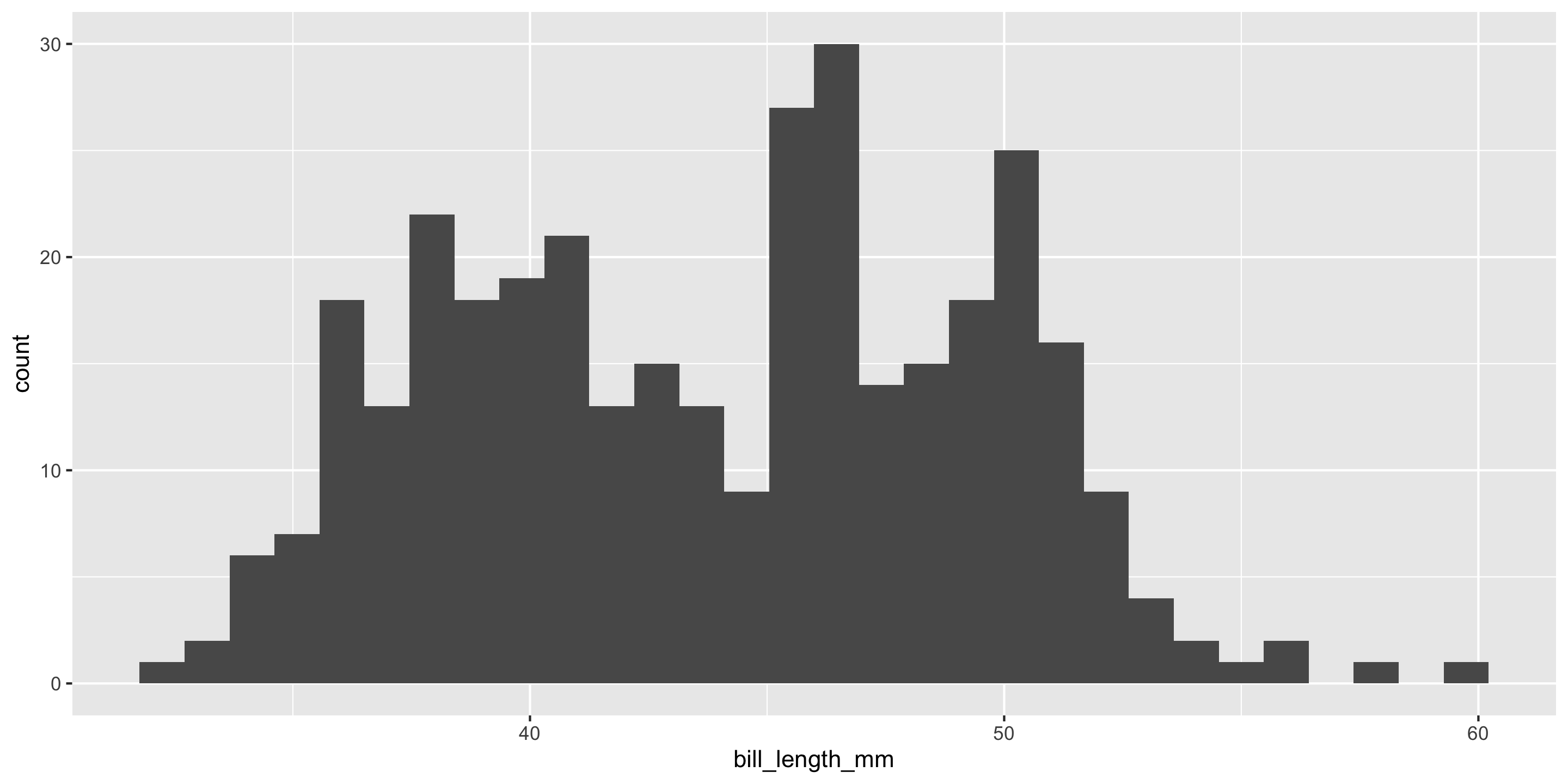
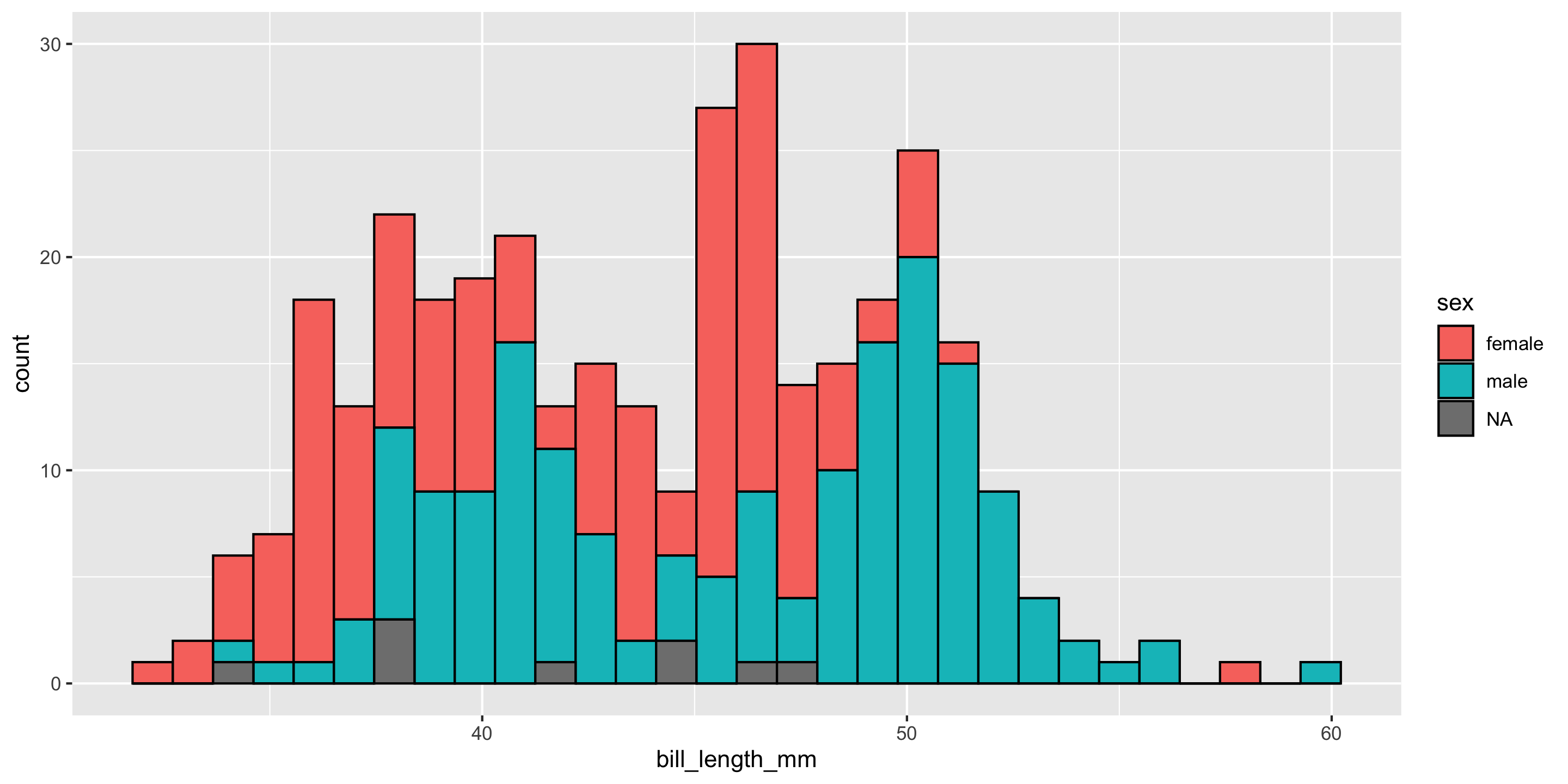
Plot A Continuous Variable
🧠 YOUR TURN
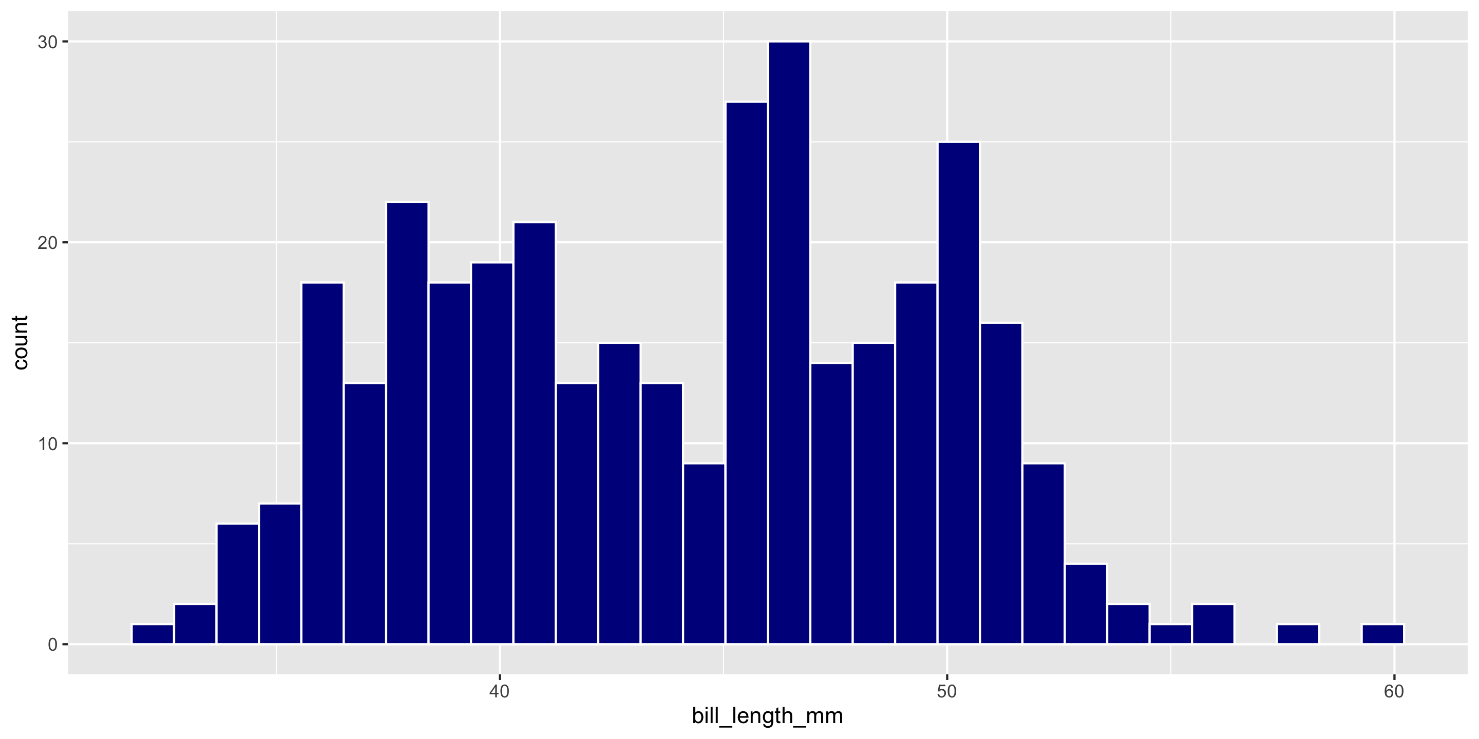
ggplot(data = penguins,
       mapping = aes(x = bill_length_mm)) +
  geom_histogram(fill = "darkblue",
color = "white")05:00
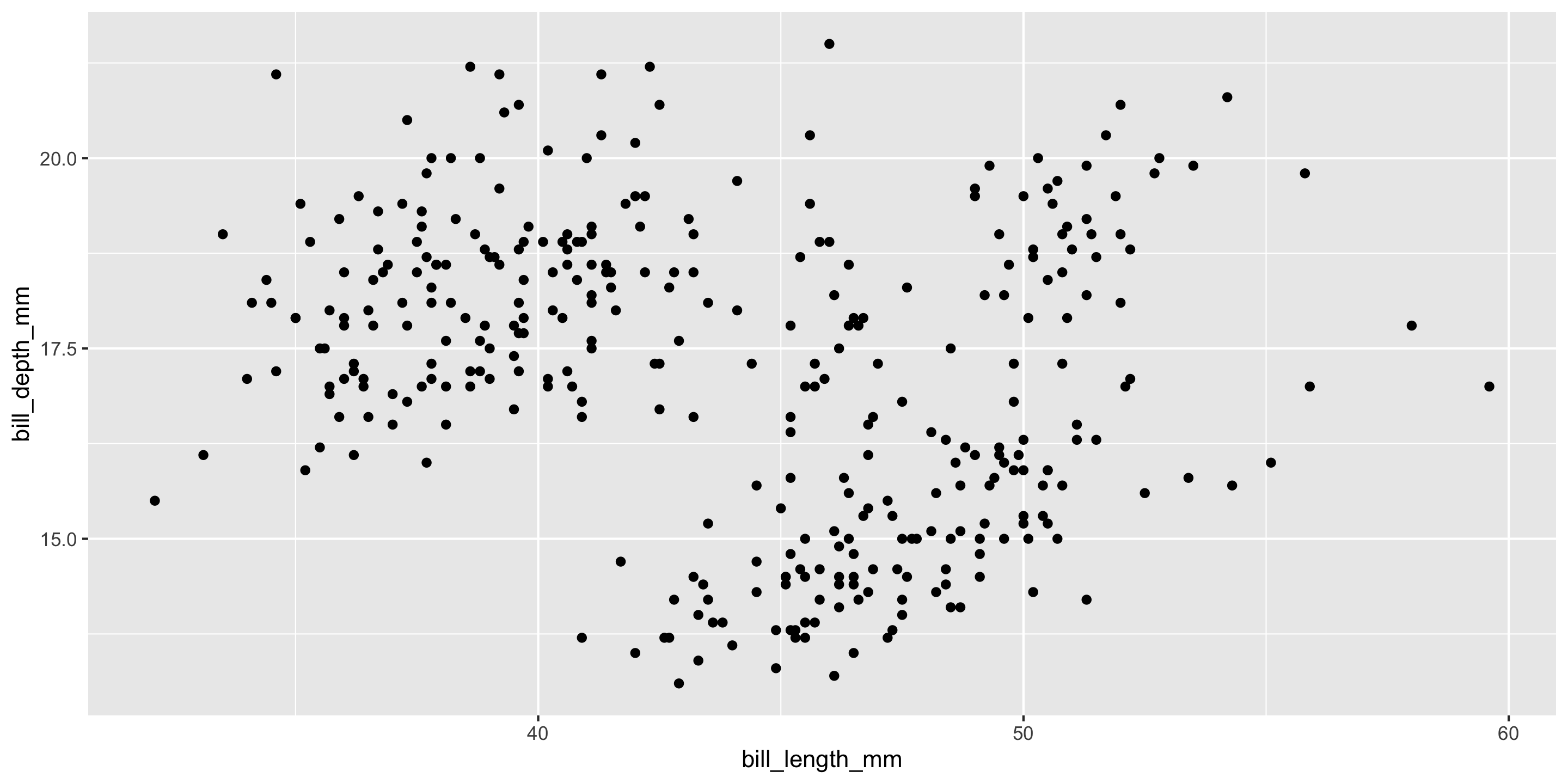
Two Continuous Variables
Geom Size
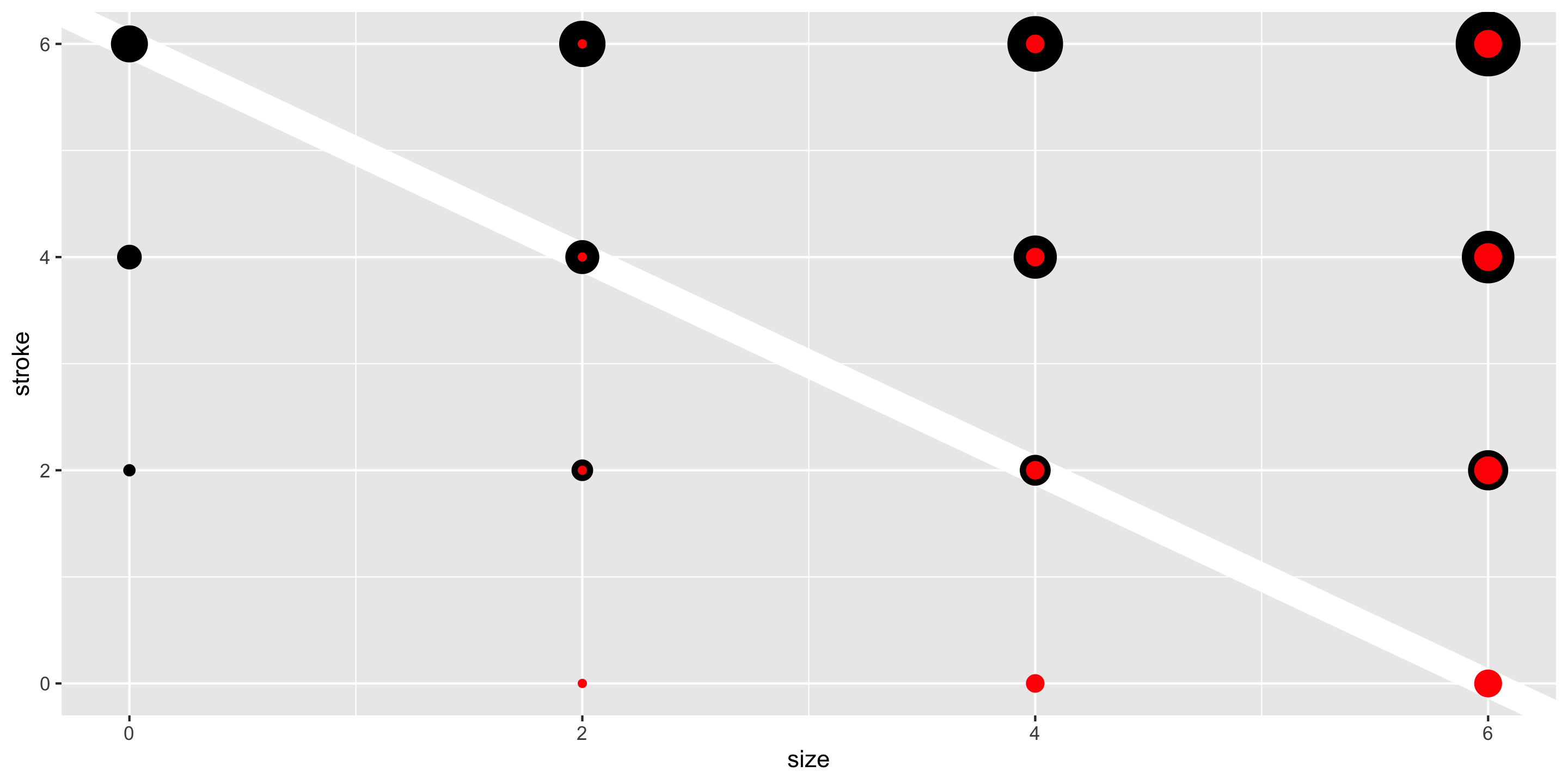

Geom Shape
🧠 YOUR TURN
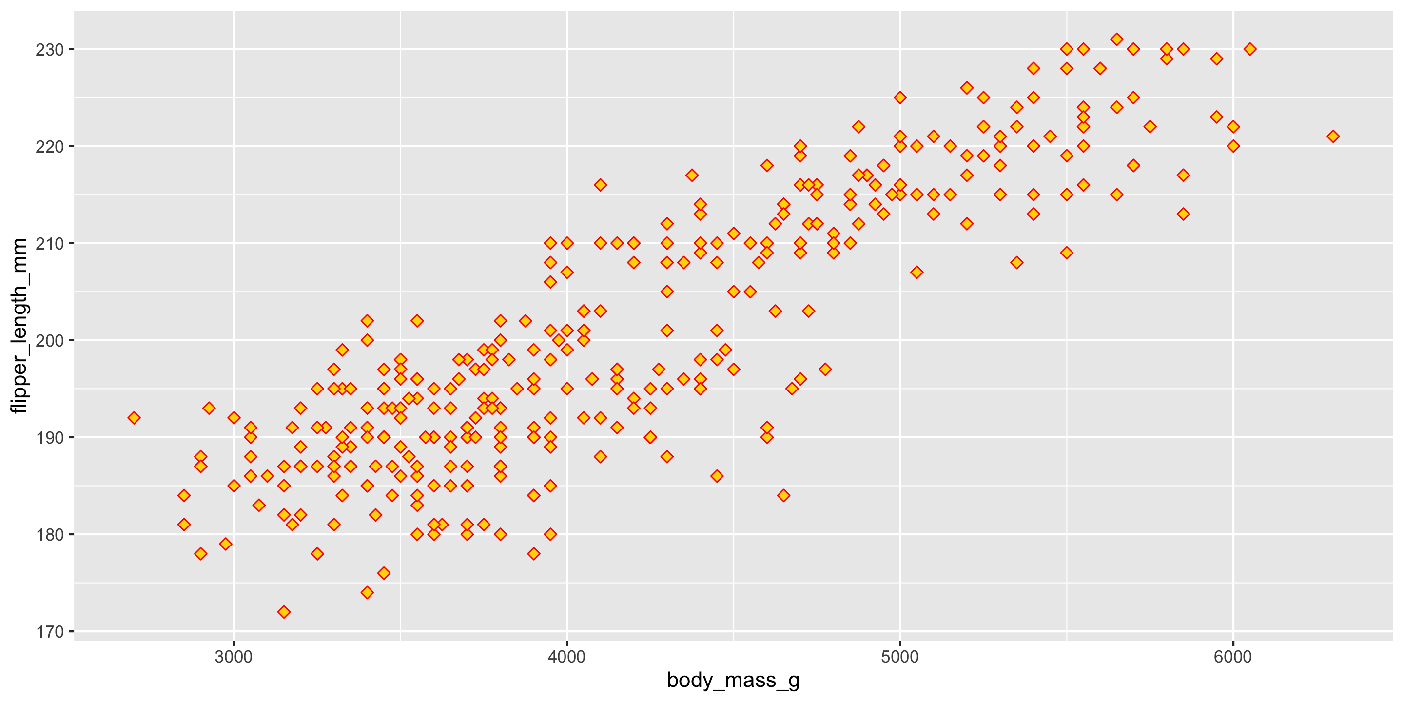
ggplot(data = penguins,
       mapping = aes(x = body_mass_g, y = flipper_length_mm)) +
geom_point(size = 2, shape = 23, color = "red", fill = "gold")05:00
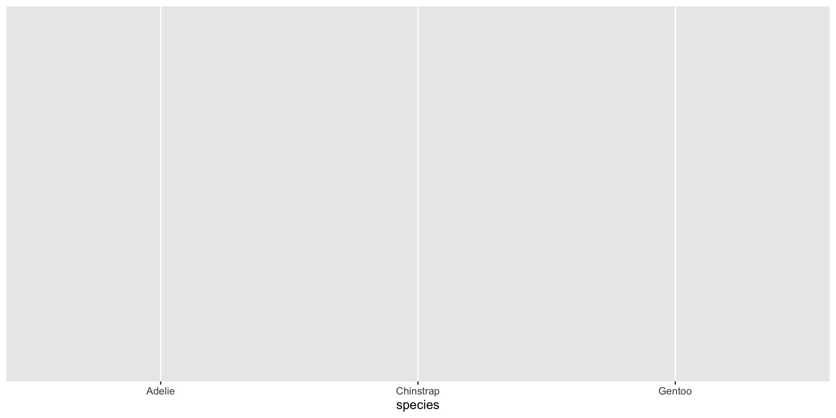
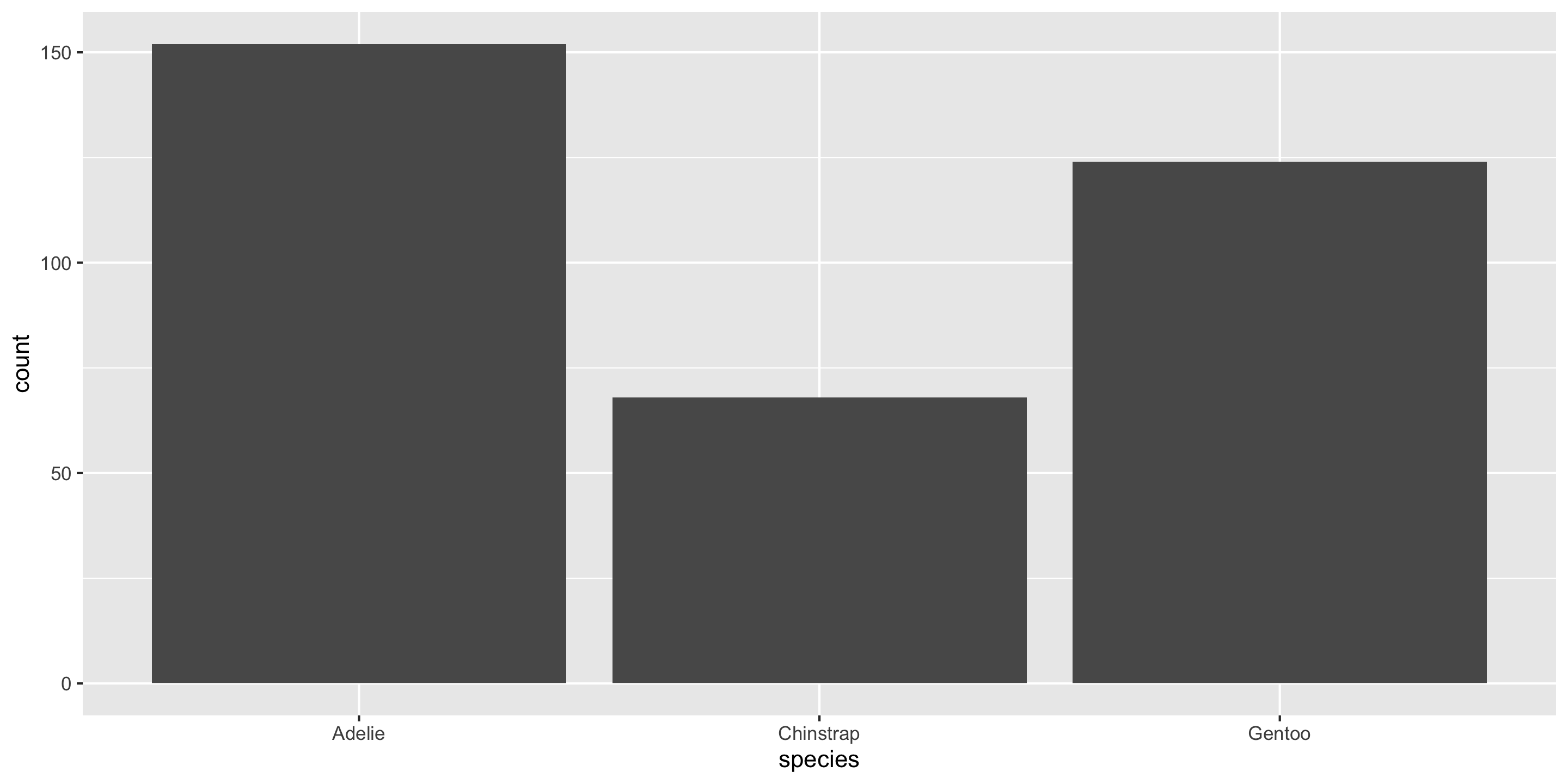
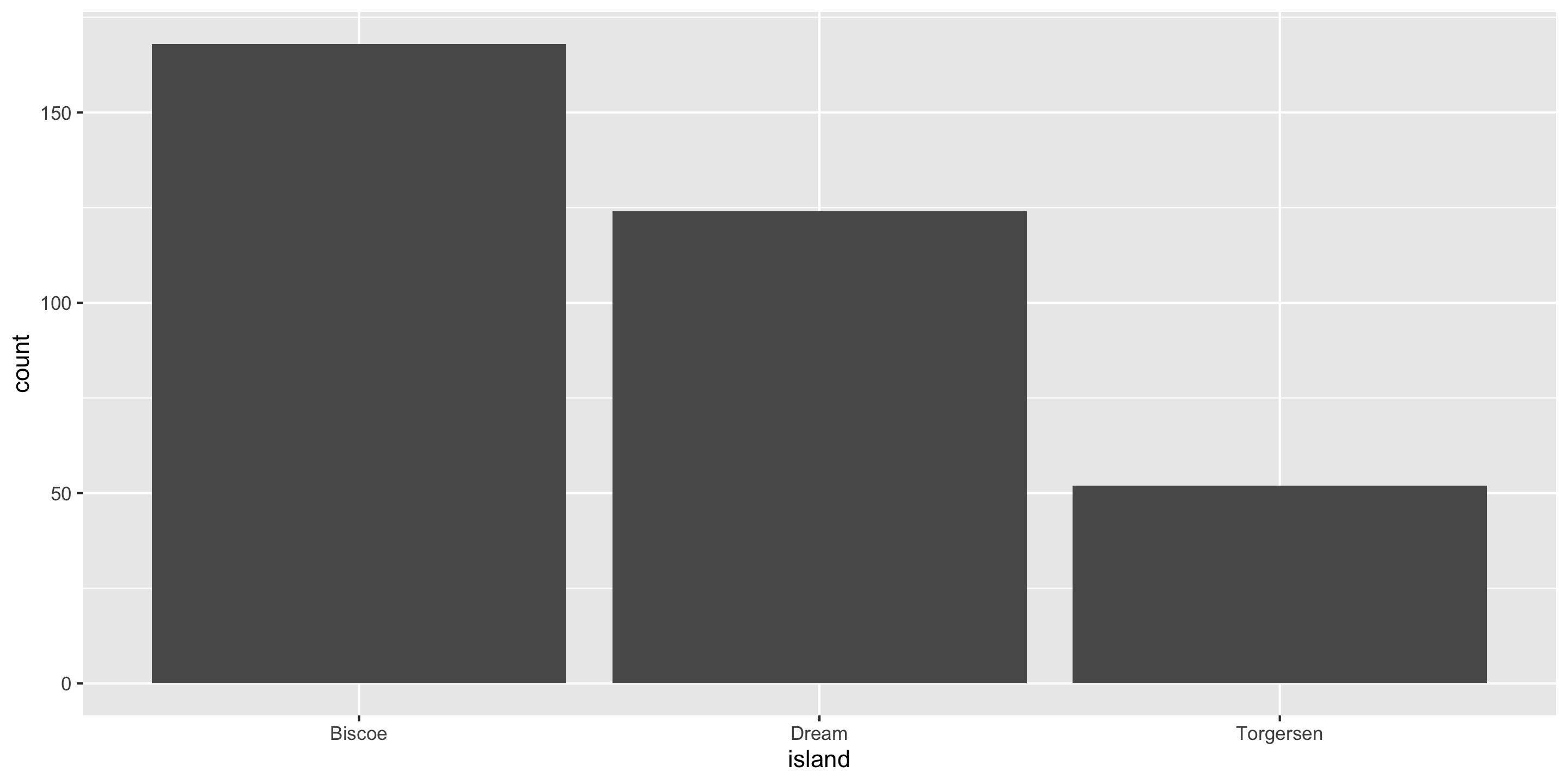
Plot A Factor & Factor
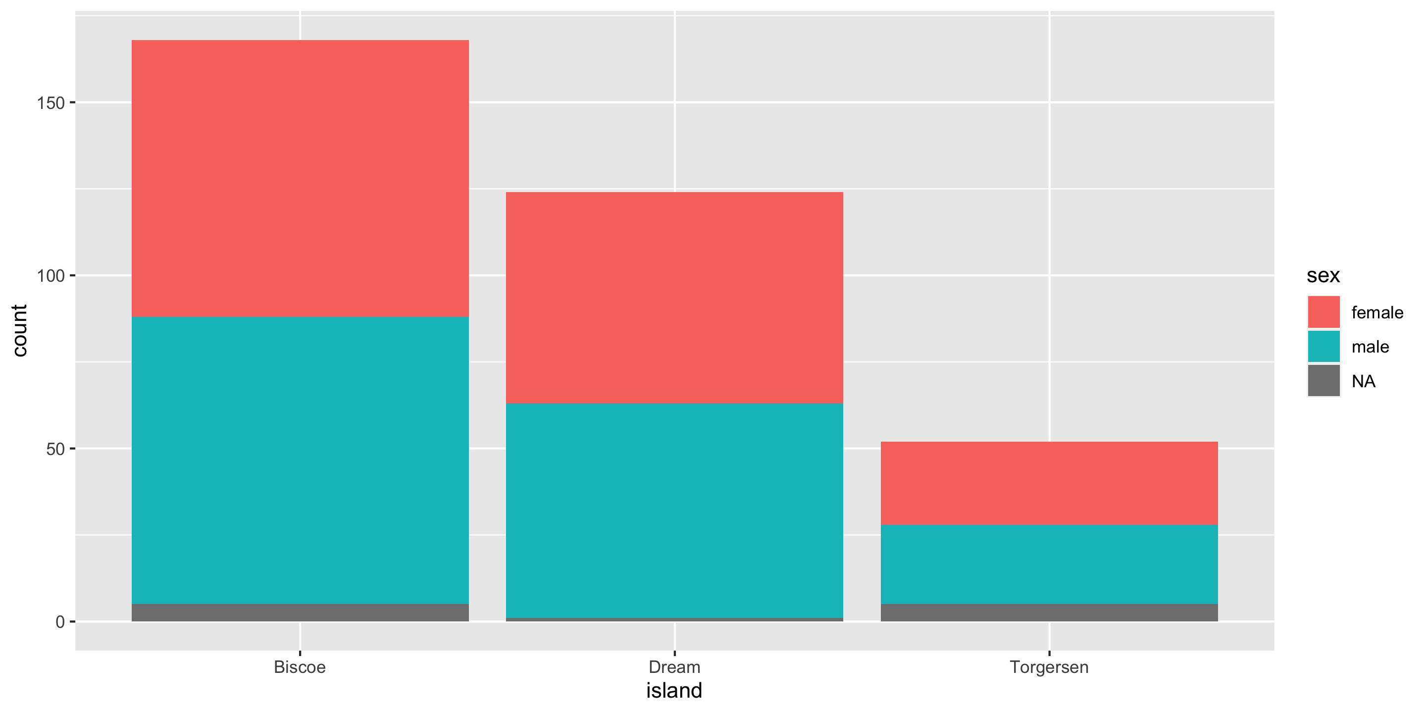
Plot A Factor & Continuous
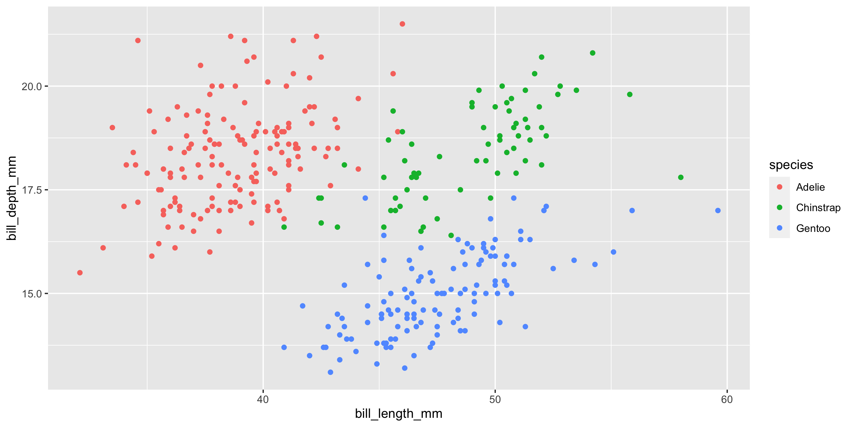
A Factor & Two Cont.
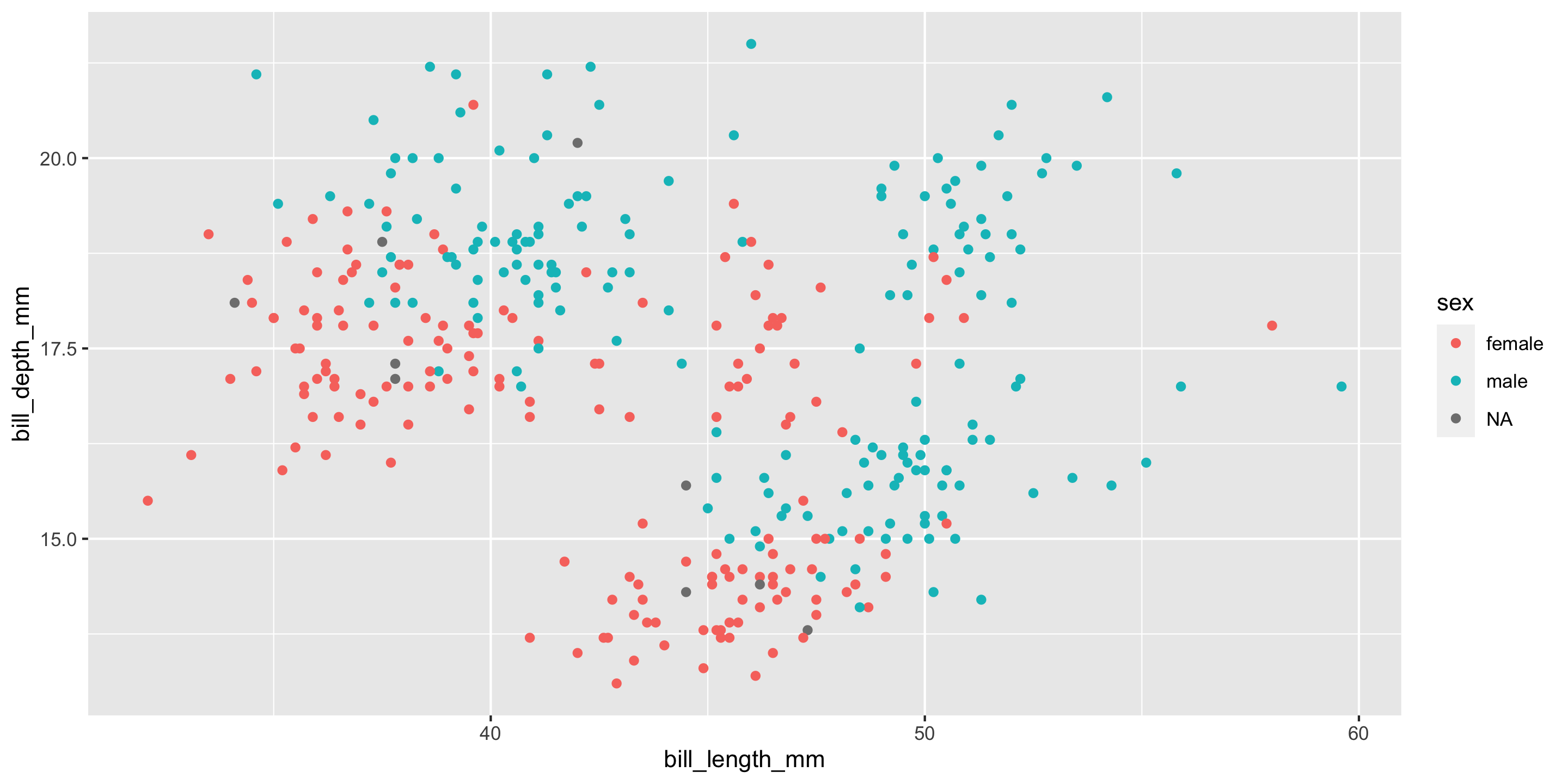
A Factor & Two Cont.
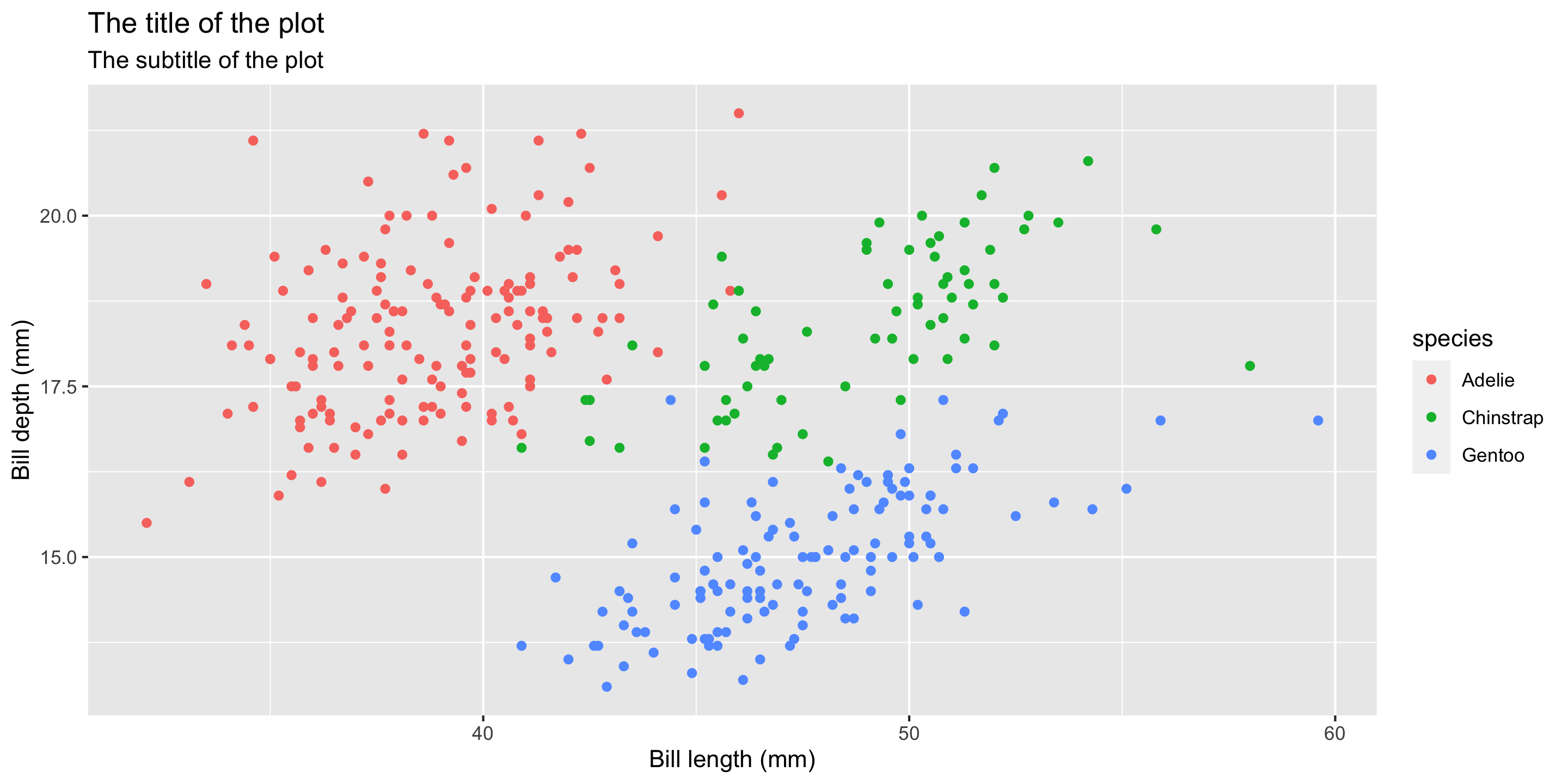
Write Labels
Title of the plot
Subtitle of the plot with more information
Title of the x-axis
Title of the y-axis
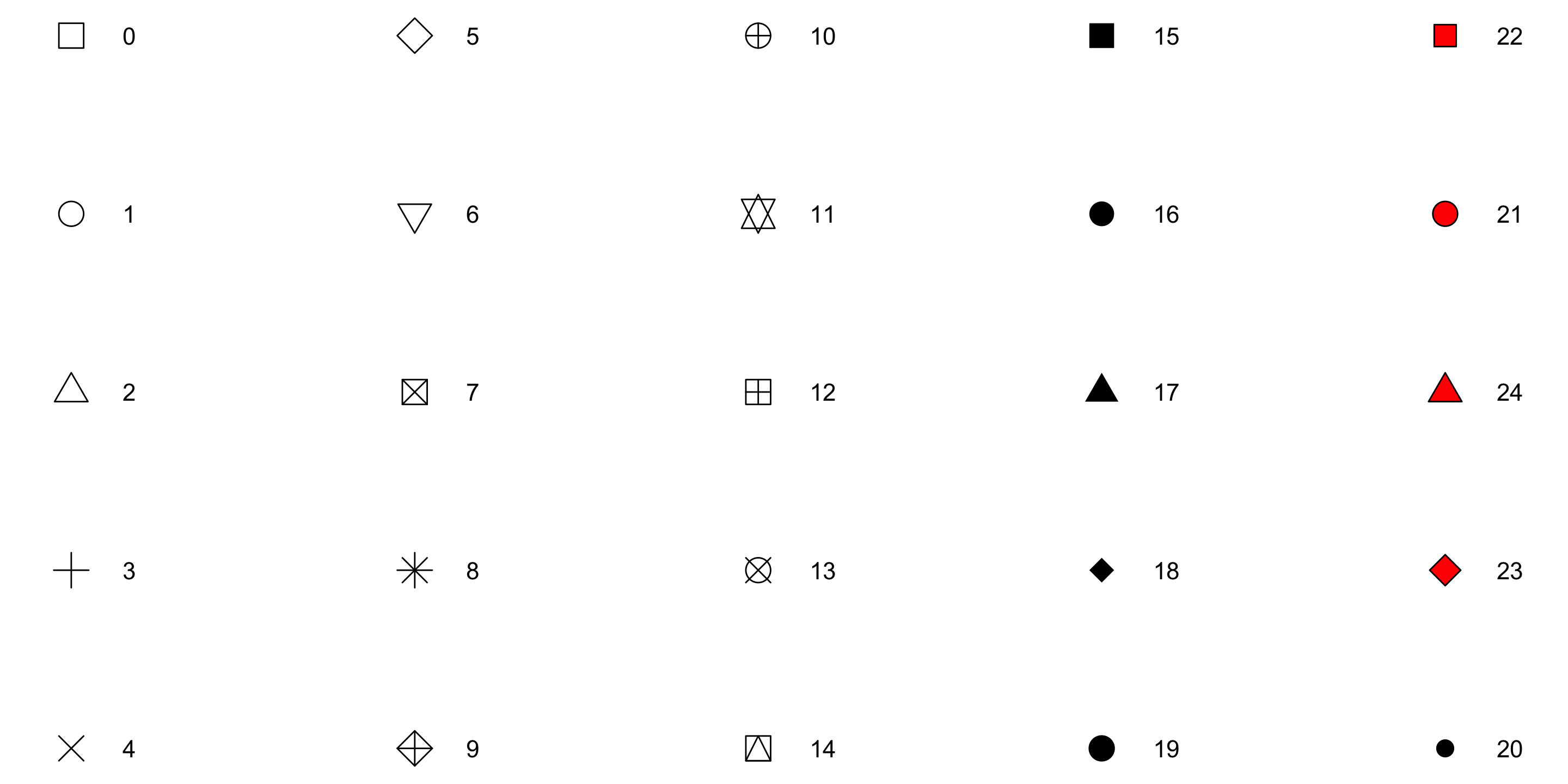
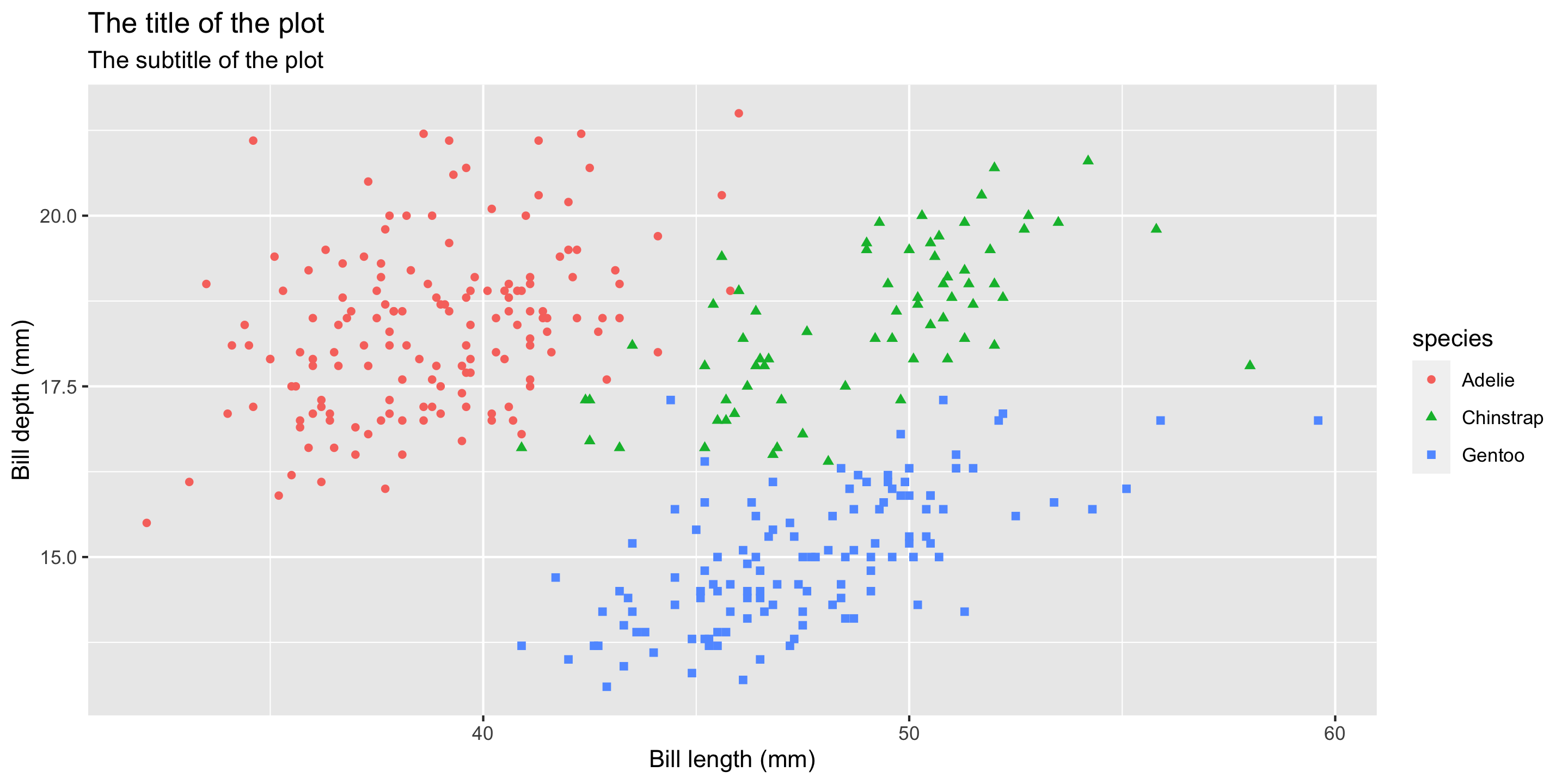
Different Shapes
Each level of the factor/category can be shown using a different shape of different color.
Various Themes
Various Themes
Various Themes
Various Themes
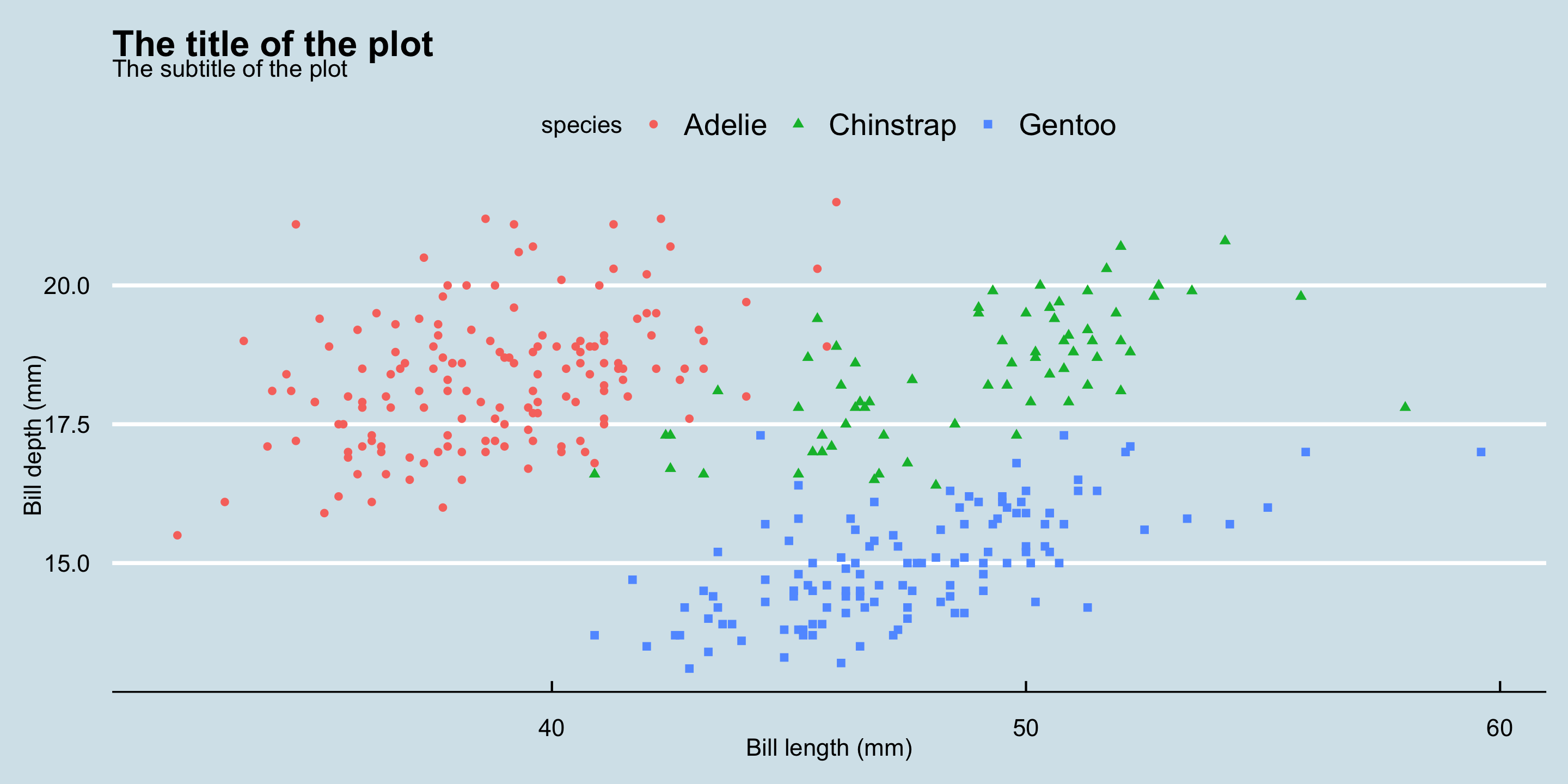
Color Palette
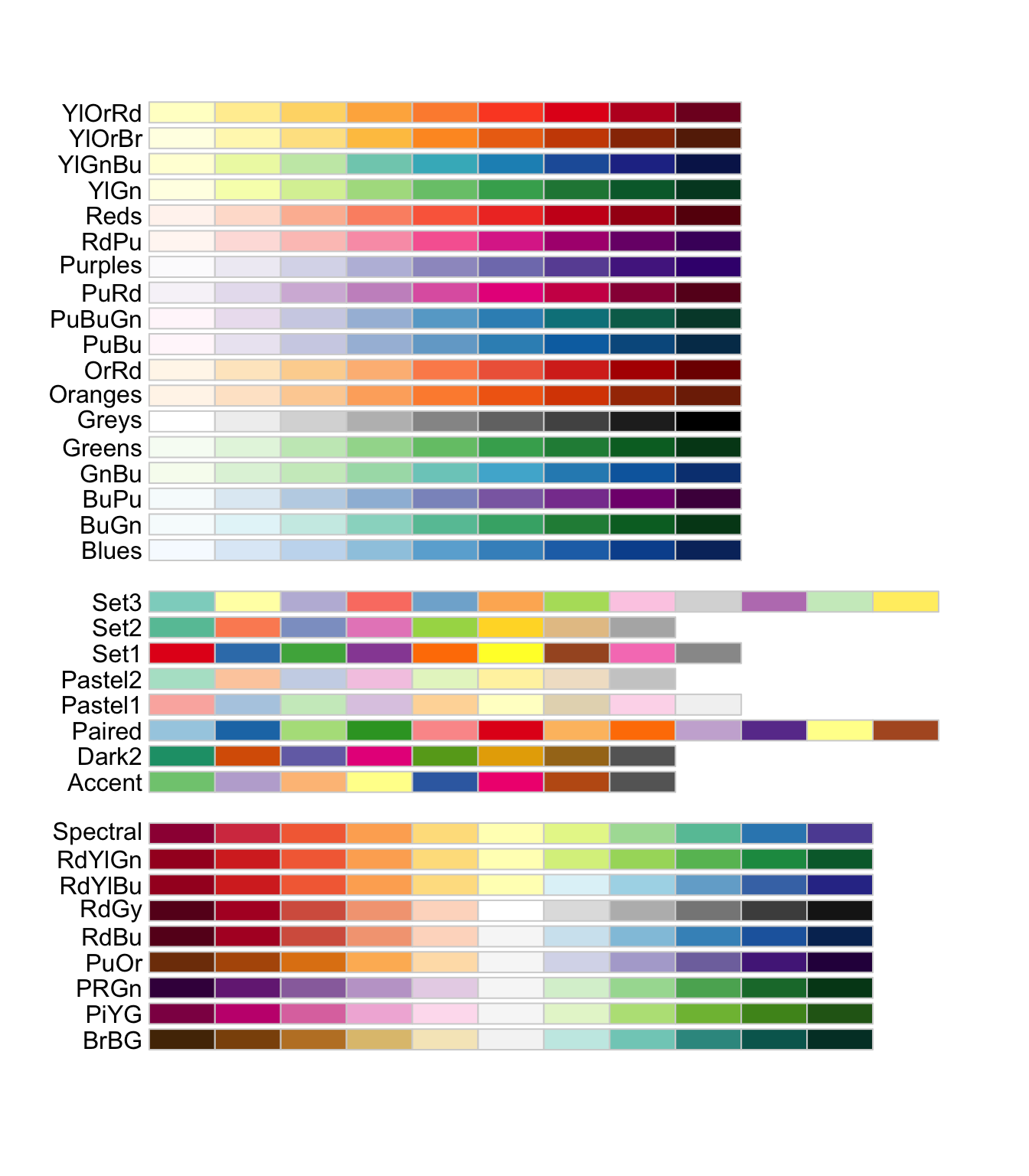
Color Palette
R package ggthemes have function to use color scheme for colorblindness. Know more
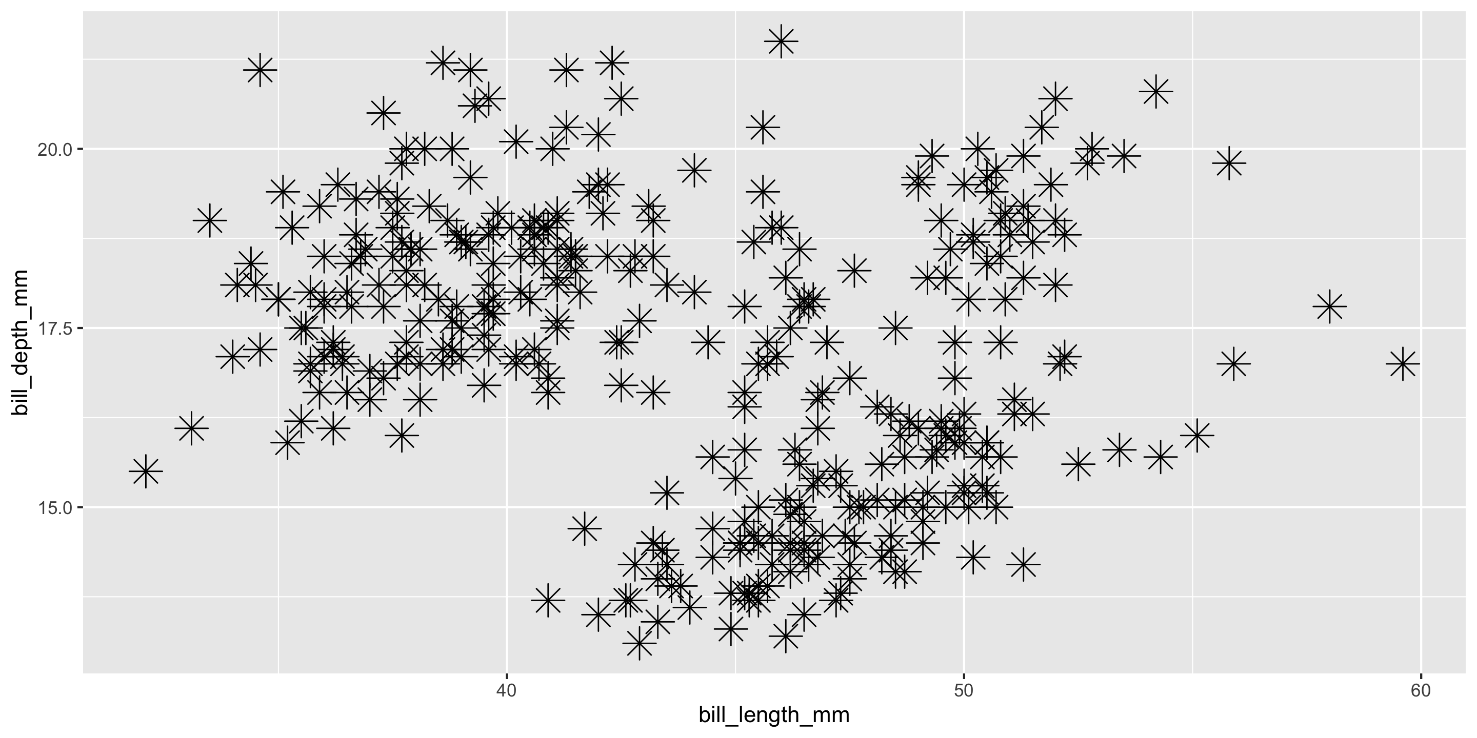
ggplot(data = penguins,
       mapping = aes(x = bill_length_mm, y = bill_depth_mm)) +
  geom_point(aes(color = species, shape = species)) +
  labs(
    title = "The title of the plot",
    subtitle = "The subtitle of the plot",
    x = "Bill length (mm)",
    y = "Bill depth (mm)"
) +
theme_clean() +
scale_color_colorblind()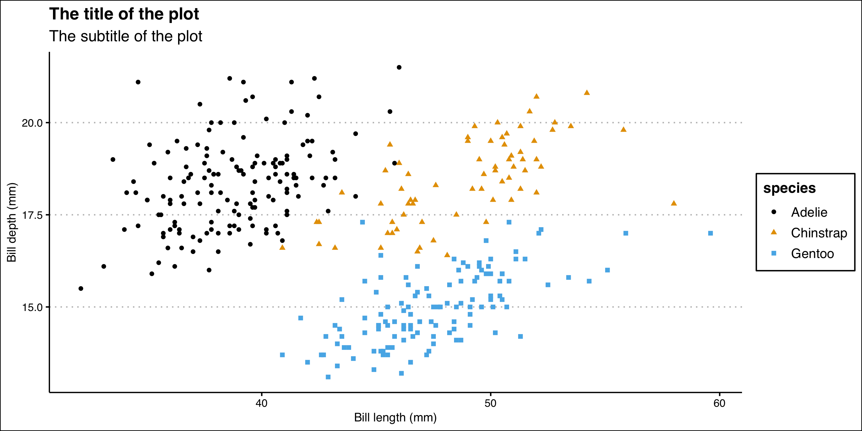
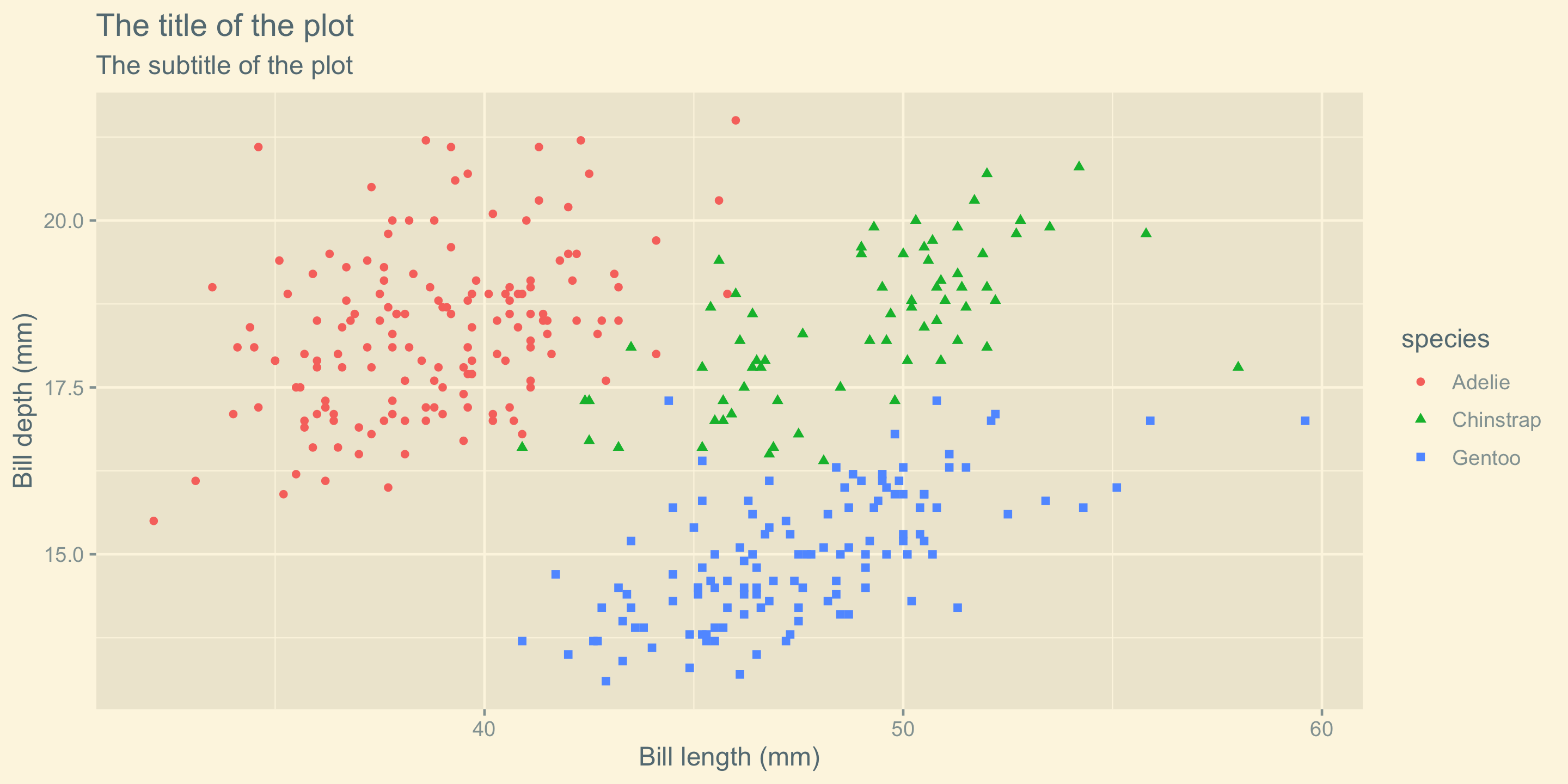
Color Palette
library(RColorBrewer)ggplot(data = penguins,
mapping = aes(x = bill_length_mm, y = bill_depth_mm)) +
geom_point(aes(color = species, shape = species)) +
labs(
title = "The title of the plot",
subtitle = "The subtitle of the plot",
x = "Bill length (mm)",
y = "Bill depth (mm)"
) +
theme_clean() +
scale_color_brewer(palette = "Dark2")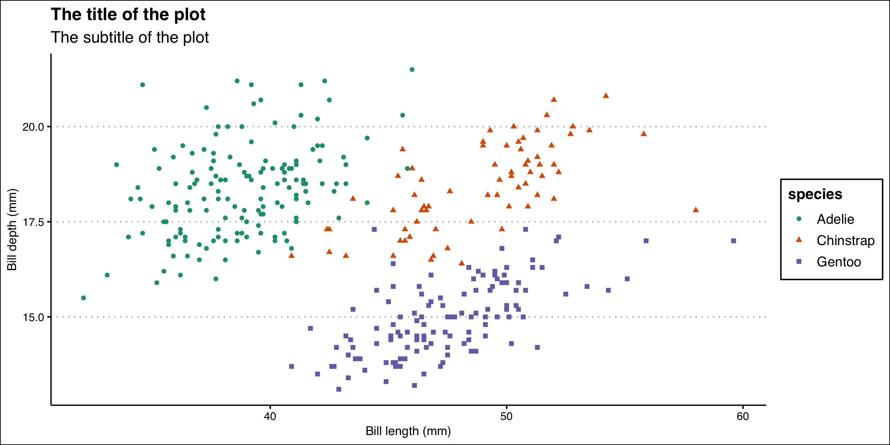
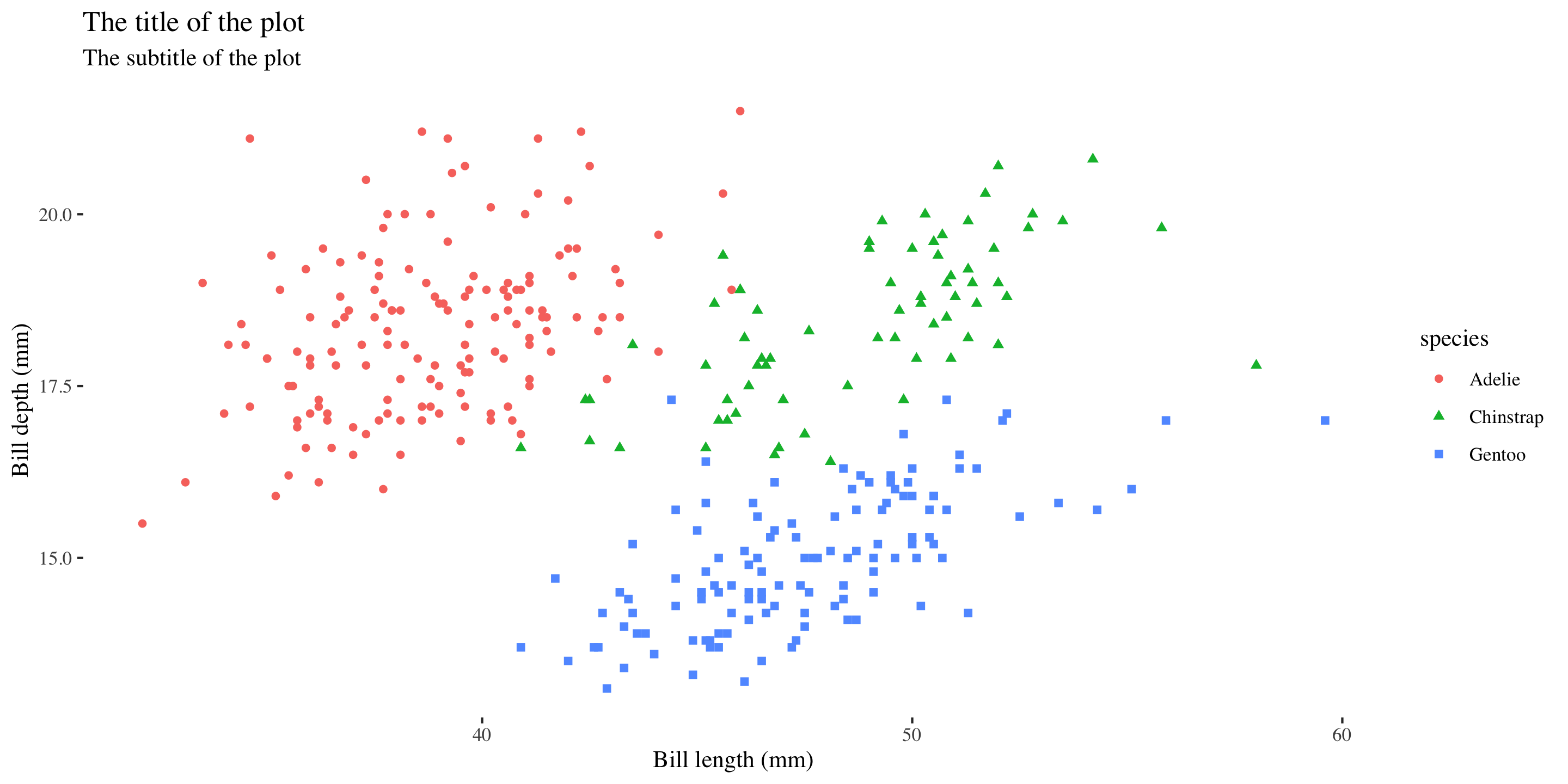
Color Palette
library(wesanderson)
names(wes_palettes) [1] "BottleRocket1" "BottleRocket2" "Rushmore1"
[4] "Rushmore" "Royal1" "Royal2"
[7] "Zissou1" "Zissou1Continuous" "Darjeeling1"
[10] "Darjeeling2" "Chevalier1" "FantasticFox1"
[13] "Moonrise1" "Moonrise2" "Moonrise3"
[16] "Cavalcanti1" "GrandBudapest1" "GrandBudapest2"
[19] "IsleofDogs1" "IsleofDogs2" "FrenchDispatch"
[22] "AsteroidCity1" "AsteroidCity2" "AsteroidCity3" ggplot(data = penguins,
mapping = aes(x = bill_length_mm, y = bill_depth_mm)) +
geom_point(aes(color = species, shape = species)) +
labs(
title = "The title of the plot",
subtitle = "The subtitle of the plot",
x = "Bill length (mm)",
y = "Bill depth (mm)"
) +
theme_clean() +
scale_color_manual(values = wes_palette("BottleRocket2", n = 3))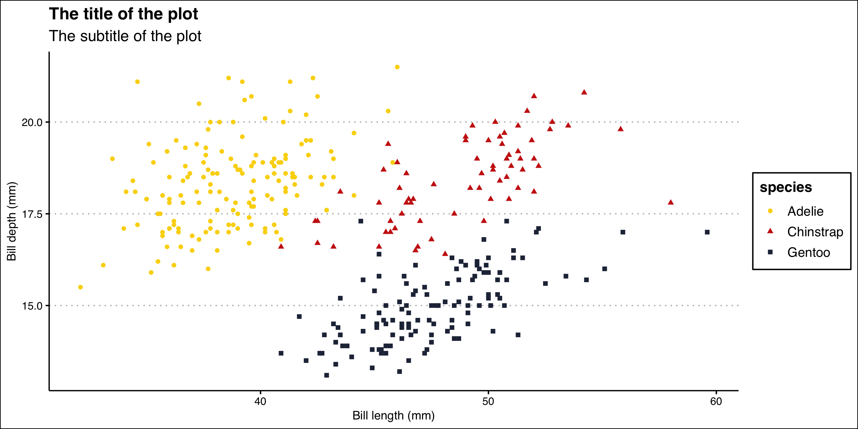
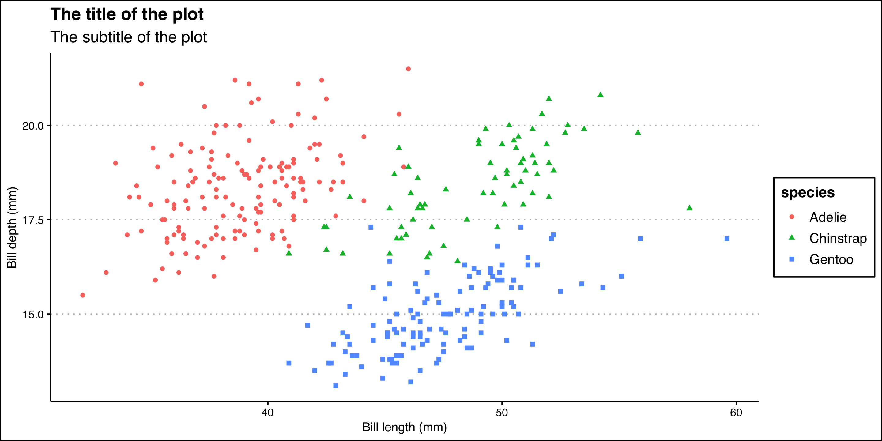
Export Plot
Export/save plot as pdf, jpg or png file.
ggplot(data = penguins,
       mapping = aes(x = bill_length_mm, y = bill_depth_mm)) +
  geom_point(aes(color = species, shape = species)) +
  labs(
    title = "The title of the plot",
    subtitle = "The subtitle of the plot",
    x = "Bill length (mm)",
    y = "Bill depth (mm)"
  ) +
theme_clean() +
scale_color_manual(values = wes_palette("BottleRocket2", n = 3))
ggsave("penguins-plot.pdf")
filter() Function:
Picks cases/observations based on their values.

filter() Function
How to have a data of only Gentoo penguins?
# A tibble: 124 × 8
   species island bill_length_mm bill_depth_mm flipper_length_mm body_mass_g
   <fct>   <fct>           <dbl>         <dbl>             <int>       <int>
 1 Gentoo  Biscoe           46.1          13.2               211        4500
 2 Gentoo  Biscoe           50            16.3               230        5700
 3 Gentoo  Biscoe           48.7          14.1               210        4450
 4 Gentoo  Biscoe           50            15.2               218        5700
 5 Gentoo  Biscoe           47.6          14.5               215        5400
 6 Gentoo  Biscoe           46.5          13.5               210        4550
 7 Gentoo  Biscoe           45.4          14.6               211        4800
 8 Gentoo  Biscoe           46.7          15.3               219        5200
 9 Gentoo  Biscoe           43.3          13.4               209        4400
10 Gentoo  Biscoe           46.8          15.4               215        5150
# ℹ 114 more rows
# ℹ 2 more variables: sex <fct>, year <int>
filter() Function
How to have a data of penguins of bill length more than 43 mm?
penguins |>
  filter(bill_length_mm > 43)
# A tibble: 188 × 8
species island bill_length_mm bill_depth_mm flipper_length_mm body_mass_g
<fct> <fct> <dbl> <dbl> <int> <int>
1 Adelie Torgersen 46 21.5 194 4200
2 Adelie Dream 44.1 19.7 196 4400
3 Adelie Torgersen 45.8 18.9 197 4150
4 Adelie Dream 43.2 18.5 192 4100
5 Adelie Biscoe 43.2 19 197 4775
6 Adelie Biscoe 45.6 20.3 191 4600
7 Adelie Torgersen 44.1 18 210 4000
8 Adelie Torgersen 43.1 19.2 197 3500
9 Gentoo Biscoe 46.1 13.2 211 4500
10 Gentoo Biscoe 50 16.3 230 5700
# ℹ 178 more rows
# ℹ 2 more variables: sex <fct>, year <int>
select() Function:
Picks variables/columns based on their names.

mutate() Function:
Adds new variables that are functions of existing variables.
arrange() Function:
Changes the ordering of the rows.

summarise() Function:
Reduces multiple values down to a single summary.
Thank
You
![]()
Social Media #RStats
Artwork by Alision Horst